SVI and NUTS give different results

This is kind of a continuation of an earlier issue I posted a week or two ago, where I was not able to recover the distribution of a latent variable in a simple model of exponential growth. Based on the discussion in that thread, I assumed that Pyro just wasn’t able to do what I was expecting (infer the distribution of a latent variable using observations of a dependent variable), even though it seemed fairly basic.

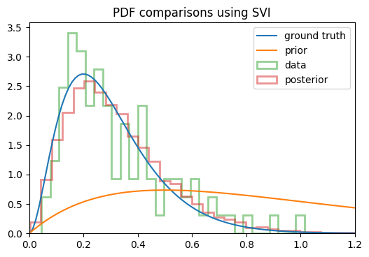
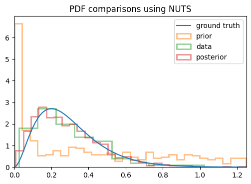
On a whim, I decided to see if MCMC could do it, so I banged out a quick trial with NUTS, and without changing the model/prior at all, I started getting the results I was expecting! You can see below the change in the posterior between using SVI vs NUTS:

svi_dist

nuts_dist

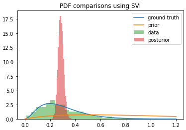
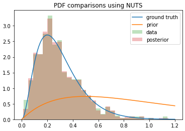
You can see that the posterior I get from SVI converges to the mean of the distribution itself (if I run it for more steps, it keeps getting narrower), whereas NUTS actually returns samples from the posterior as I was hoping. I used the same model in each case, so what’s going on here? Am I using SVI incorrectly?

You can reproduce this with the following code:

import tqdm
import numpy as np
import scipy
import matplotlib.pyplot as plt
import random

import torch
from torch.distributions import constraints as tconst
import pyro
import pyro.distributions as pdist
import pyro.infer
from pyro.infer import MCMC, NUTS, Predictive
import pyro.optim

pyro.enable_validation(True)


####################################################################
##                       Define model/guide                       ##
####################################################################


class RegressionModel:
    def __init__(self, k, theta):
        self.k = torch.tensor(float(k))
        self.theta = torch.tensor(float(theta))
        
    # Model used in both SVI and NUTS
    def model(self, Y):
        for i, y in enumerate(Y):
            N = len(y) - 1
            noise = 1e-3
            with pyro.plate(f"data_{i}", N):
                r = pyro.sample(f"r_{i}", pdist.Gamma(self.k, 1/self.theta))
                ln_yhat = torch.log(1+r) + torch.log(y[:-1])
                pyro.sample(f"obs_{i}", pdist.Normal(ln_yhat, noise), obs=torch.log(y[1:]))
    
    # Guide only used for SVI
    def guide(self, Y):
        for i, y in enumerate(Y):
            N = len(y) - 1
            k = pyro.param("k", self.k, constraint=tconst.positive)
            theta = pyro.param("theta", self.theta, constraint=tconst.positive)
            with pyro.plate(f"data_{i}", N):
                r = pyro.sample(f"r_{i}", pdist.Gamma(k, 1/theta))
                

####################################################################
##                       Generate data                            ##
####################################################################

K, THETA = 3e0, 1e-1  # Actual ground truth values
def gen_ts(k, theta, T=10):
    y0 = 1
    Y = [y0]
    for t in range(T):
        y0 = (1 + random.gammavariate(k, theta))*y0
        Y.append(y0)
    return torch.tensor(Y)

# Make a bunch of time series of varying lengths
data = [gen_ts(K, THETA, T) for T in np.random.uniform(1, 10, size=100).round().astype(int)]


####################################################################
##                         Run SVI                                ##
####################################################################

pyro.clear_param_store()
model = RegressionModel(2, 0.5)
svi = pyro.infer.SVI(
    model=model.model,
    guide=model.guide,
    optim=pyro.optim.Adam({"lr": 1e-1, "betas": (0.9, 0.9)}),
    loss=pyro.infer.Trace_ELBO()
)

num_steps = 200
pbar = tqdm.notebook.tqdm(total=num_steps, mininterval=1)
loss = [] # For tracking loss
ps = pyro.get_param_store()
params = dict() # For tracking variational parameter evolution
alpha = 0.9 # For exponential weighted average of loss
for i in range(num_steps):
    loss.append(svi.step(data))
    if i == 0 or np.isinf(avg_loss):
        avg_loss = loss[-1]
    else:
        avg_loss = alpha * avg_loss + (1-alpha) * loss[-1]
    for k in ps.keys():
        try:
            params[k].append(ps[k].item())
        except KeyError:
            params[k] = [ps[k].item()]
    pbar.set_description(f"loss={avg_loss: 5.2e}")
    pbar.update()
pbar.close()


####################################################################
##                   Plot posterior from SVI                      ##
####################################################################

# Ground-truth distribution
x = np.linspace(0, 1.2, 100)
y = scipy.stats.gamma(a=K, scale=THETA).pdf(x)
plt.plot(x, y, label="ground truth")
# Prior distribution
x = np.linspace(0, 1.2, 100)
y = scipy.stats.gamma(a=model.k.item(), scale=model.theta.item()).pdf(x)
plt.plot(x, y, label="prior")
# Data distribution
X = []
for Y in data:
    x = ((torch.roll(Y, -1) - Y)/Y).numpy()[:-1]
    X.extend(x)
plt.hist(X, bins=30, alpha=0.5, label="sample", density=True)
# The posterior distribution
k = pyro.param('k').item()
theta = pyro.param("theta").item()
x = np.random.gamma(k, theta, size=10000)
plt.hist(x, bins=30, alpha=0.5, label="posterior", density=True)

plt.legend()
plt.title("PDF comparisons using SVI")
plt.show()

####################################################################
##                           Run NUTS                             ##
####################################################################

model = RegressionModel(2, 0.5)

nuts_kernel = NUTS(
    model.model,
    adapt_step_size=True,
    adapt_mass_matrix=True,
    jit_compile=False,
    full_mass=True
)
mcmc = MCMC(
    nuts_kernel,
    num_samples=20,
    warmup_steps=10,
    num_chains=1
)
mcmc.run(data)
samples = mcmc.get_samples()

####################################################################
##                   Plot posterior from NUTS                     ##
####################################################################


# Ground-truth distribution
x = np.linspace(0, 1.2, 100)
y = scipy.stats.gamma(a=K, scale=THETA).pdf(x)
plt.plot(x, y, label="ground truth")
# Prior distribution
x = np.linspace(0, 1.2, 100)
y = scipy.stats.gamma(a=model.k.item(), scale=model.theta.item()).pdf(x)
plt.plot(x, y, label="prior")
# Data distribution
X = []
for Y in data:
    x = ((torch.roll(Y, -1) - Y)/Y).numpy()[:-1]
    X.extend(x)
plt.hist(X, bins=30, alpha=0.3, label="data", density=True)
# Posterior samples
samples_flattened = torch.cat([s.flatten() for s in samples.values()]).numpy()
plt.hist(samples_flattened, bins=30, alpha=0.3, label="posterior", density=True)

plt.legend()
plt.title("PDF comparisons using NUTS")
plt.show()

@physicswizard I think the issue is MCMC learns a latent variable r_i for each data point, while SVI learns a single pair of latent variables k and theta for all data.

@fehiepsi I don’t think that’s it. k and theta are trainable variational hyperparameters, not latent variables. Also, I made a different k and theta for each data point and ran SVI again and each of the individual parameters follows the same pattern. I also ran both NUTS/SVI on a single data point (technically single time series) and got the same behavior as before.

The model I want to specify is one where there is a single distribution R which is sampled from multiple times to get different samples r for each data point, so I think I do want a single pair of (k,theta). NUTS learns similar distributions for all the sample sites because they should be iid anyway; all the r's are drawn from the same distribution.

have you plotted 2d density plots for slices of the approximate posterior returned by NUTS, e.g. r[i] versus r[i+1] for various i? i wouldn’t expect these to be well approximated by mean field gaussian distributions

I don’t think I can, the different r[i] are of potentially different lengths

@martinjankowiak @fehiepsi I think I figured it out; my problem basically stemmed from my own fundamental misunderstanding about how SVI/HMC worked. I believe that the problem was 1) I was sampling then applying deterministic transformations to the samples, rather than the other way around, and 2) I was creating multiple latent variables as @fehiepsi had pointed out, when I really only wanted multiple samples from the same distribution. Using TransformedDistribution was critical to resolving problem #1, and I had to move some things in/out of pyro.plate to resolve #2.

Here are my new models/guides:

class SVIModel:
    """
    This models the system of equations y_{i+1} = (1+r)*y_i, where r ~ Gamma(k, theta).
    The object is to perform inference and reconstruct the distribution of r using SVI
    (which means recovering the parameters k and theta).
    """
    def __init__(self, k, theta):
        # Specify the parameters of the prior, and also the starting
        # values of the variational parameters
        self.k = torch.tensor(float(k))
        self.theta = torch.tensor(float(theta))

    def model(self, y):
        N = len(y) - 1
        # K and theta are variational parameters, but we still need to "sample" them
        k = pyro.sample("k_", Delta(self.k))
        theta = pyro.sample("theta_", Delta(self.theta))
        with pyro.plate("data", N):
            # Now we need to specify the distribution of the target in terms
            # of transformed distributions
            x = Gamma(k, 1/theta) # The original distribution for r
            x = TransformedDistribution(x, AffineTransform(1., 1.)) # 1+r
            x = TransformedDistribution(x, ExpTransform().inv) # log(1+r)
            X, Y = torch.log(y[:-1]), torch.log(y[1:])
            Yhat = TransformedDistribution(x, AffineTransform(X, 1.)) # log(1+r) + log(y_i)
            obs = pyro.sample("obs", Yhat, obs=Y)

    def guide(self, y):
        N = len(y) - 1
        k = pyro.param("k", self.k, constraint=tconst.positive)
        theta = pyro.param("theta", self.theta, constraint=tconst.positive)
        # Even though k and theta aren't random variables, we still need
        # to sample them so the guide knows it needs to optimize them
        pyro.sample("k_", Delta(k))
        pyro.sample("theta_", Delta(theta))

    def r(self, N=1):
        # Useful for sampling from the posterior of r
        k = pyro.param("k", self.k, constraint=tconst.positive)
        theta = pyro.param("theta", self.theta, constraint=tconst.positive)
        return Gamma(k, 1/theta).sample([N])


class HMCModel:
    """
    This models the system of equations y_{i+1} = (1+r)*y_i, where r ~ Gamma(k, theta).
    The object is to perform inference and reconstruct the distribution of r using HMC (NUTS).
    This actually means recovering the posterior of the parameters of the gamma distribution
    which determines r.
    """
    def __init__(self, k, theta):
        # Specify the parameters of the prior
        self.k = torch.tensor(float(k))
        self.theta = torch.tensor(float(theta))

    def model(self, y):
        N = len(y) - 1
        # Sample from the hyperpriors for r
        alpha = abs(pyro.sample("k", Uniform(0, 4)))
        beta = 1/abs(pyro.sample("theta", Uniform(0, 3)))
        with pyro.plate("data", N):
            # Now we need to specify the distribution of the target in terms
            # of transformed distributions
            r = Gamma(alpha, beta) # The original distribution for r
            x = TransformedDistribution(r, AffineTransform(1., 1.)) # 1+r
            x = TransformedDistribution(x, ExpTransform().inv) # log(1+r)
            X, Y = torch.log(y[:-1]), torch.log(y[1:])
            Yhat = TransformedDistribution(x, AffineTransform(X, 1.)) # log(1+r) + log(y_i)
            obs = pyro.sample("obs", Yhat, obs=Y)

Here are the results for the distribution of the growth rate r:

svi_distributions

nuts_distributions

Appreciate your guys’ help! I’m still a noob when it comes to Bayesian inference and probabilistic programming, so this struggle has been very educational for me :slight_smile:

3 Likes