Distribution is converging to the mean

I am trying to do a regression on some exponential growth data just as a toy example. My data is generated via y_{t+1} = (1+r_t) y_t, where r_t is sampled from a gamma distribution to enforce positivity (and y_0=1). I can turn this into linear regression by taking the log, so I get a model like \ln(y_{t+1}) = \ln(1+r_t) + \ln(y_t), and although I’ve been able to do normal Bayesian linear regression (following along with the tutorial) where all distributions involved are normally distributed, this one is proving more difficult, perhaps because of some unforeseen quirk of the gamma distribution?

Anyway, the problem I’m having is that when trying to get the posterior for r_t, the density seems to converge toward the correct mean, but the variance keeps shrinking the longer I train. The ELBO loss continues to decrease as though training is proceeding correctly, but the posterior is clearly getting worse as time goes on.

elbo
parameter_evolution
posterior

My model is currently set up as below:

import tqdm
import numpy as np
import matplotlib.pyplot as plt
import random

import torch
from torch.distributions import constraints as tconst
import pyro
from pyro.nn import PyroModule, PyroParam, PyroSample
import pyro.distributions as pdist
import pyro.infer
import pyro.optim

class RegressionModel:
    def __init__(self, mean, std):
        super().__init__()
        # Convert mean/std into parameters of the gamma dist.
        k = (mean/std)**2
        theta = (std**2)/mean
        # k and theta will themselves be gamma distributed
        self.k_mean = torch.tensor(float(k))
        self.k_std = torch.tensor(float(k))
        self.theta_mean = torch.tensor(float(theta))
        self.theta_std = torch.tensor(float(theta))
        
        self.k_k = (self.k_mean/self.k_std)**2
        self.k_theta = (self.k_std**2)/self.k_mean
        self.theta_k = (self.theta_mean/self.theta_std)**2
        self.theta_theta = (self.theta_std**2)/self.theta_mean
    
    def model(self, y):
        N = len(y)-1
        sigma = 1e-5
        with pyro.plate("data", N):
            k = pyro.sample("k", pdist.Gamma(self.k_k, 1/self.k_theta))
            theta = pyro.sample("theta", pdist.Gamma(self.theta_k, 1/self.theta_theta))
            r = pyro.sample("r", pdist.Gamma(k, 1/theta))
            # Need to perform log transform to get additive noise
            ln_yhat = torch.log(1+r) + torch.log(y[:-1])
            pyro.sample(f"obs", pdist.Normal(ln_yhat, sigma), obs=torch.log(y[1:]))
        
    def guide(self, y):
        N = len(y)-1
        k_k = pyro.param("k_k", self.k_k, constraint=tconst.positive)
        k_theta = pyro.param("k_theta", self.k_theta, constraint=tconst.positive)
        theta_k = pyro.param("theta_k", self.theta_k, constraint=tconst.positive)
        theta_theta = pyro.param("theta_theta", self.theta_theta, constraint=tconst.positive)
        with pyro.plate("data", N):
            k = pyro.sample("k", pdist.Gamma(k_k, 1/k_theta))
            theta = pyro.sample("theta", pdist.Gamma(theta_k, 1/theta_theta))
            r = pyro.sample("r", pdist.Gamma(k, 1/theta))

There is one gamma distribution for the growth rate r, and one gamma distribution each for the hyperparameters k and \theta of the r distribution. The training/fitting procedure is as follows:

## Generate dataset
K, THETA = 10, 0.01
y0 = 1
Y = [y0]
for t in range(500):
    y0 = (1 + random.gammavariate(K, THETA))*y0
    Y.append(y0)
Y = torch.tensor(Y)

pyro.enable_validation(True)
pyro.clear_param_store()
model = RegressionModel(0.1, 0.1)
svi = pyro.infer.SVI(
    model=model.model,
    guide=model.guide,
    optim=pyro.optim.Adam({"lr": 1e-3, "betas": (0.9, 0.9)}),
    loss=pyro.infer.Trace_ELBO()
)

num_steps = 20000
pbar = tqdm.notebook.tqdm(total=num_steps, mininterval=1)
loss = []
ps = pyro.get_param_store()
params = {k: [] for k in ['k_k', 'k_theta', 'theta_k', 'theta_theta']}
alpha = 0.99
for _ in range(num_steps):
    loss.append(svi.step(Y))
    for k in ps.keys():
        params[k].append(ps[k].item())
    try:
        avg_loss = alpha * avg_loss + (1-alpha) * loss[-1]
    except:
        avg_loss = loss[-1]
    pbar.set_description(f"loss={avg_loss: 5.2e}")
    pbar.update()
pbar.close()

Is there something simple that I am overlooking? Or have a made some grave mistake? Is this a known shortcoming of using gamma distributions?

are you sure you want your k and theta variables inside the plate?

Pretty sure; I want a different sample for every data point in my dataset. Anyway, I tried placing it outside, and got the same results.

wouldn’t you expect the variance to be small given the very small value of sigma?

No, I only added sigma because that’s just some hack I had to do to get everything to work. Let me explain what I’m trying to do in some more detail.

I have some time-series data y_t, which can be modeled as noisy exponential growth, so that y_{t+1} = (1 + r_t) y_t. This relationship is completely deterministic, but the r_t are assumed to be iid samples from some distribution. I want to figure out what that distribution looks like.

In my toy example, I’ve been generating r_t from a gamma distribution parametrized with a fixed k and \theta$. In my third plot, you can see a histogram of like 10,000 samples from this distribution in blue, and then maybe another 100 or so in orange that I am using as the samples to fit the variational parameters k and \theta in my guide/posterior (I actually made k and \theta distributions themselves in my example in the hopes that would change things, but it didn’t, so ignore that).

After performing SVI, I would have hoped that the variational parameters for k and \theta would have converged towards their ground truth values so that I could recover the actual distribution of the r_t, but as you can see from the 2nd plot, that is not the case. When sampling from the variational posterior that I get using those parameters, I get the green distribution in the 3rd plot, which is spot-on for the mean of the ground-truth distribution, but the variance is way too low.

The only reason I’m using sigma is because that relationship between y_t and y_{t+1} is deterministic, but I couldn’t figure out a way to apply an observation of y_{t+1} in a deterministic manner (rather than observing a sample from a distribution, as is normally done). I tried using the Delta distribution, but that leads to infinite ELBO loss (I assume because the delta distribution is infinitely narrow), so I did the next best thing I could think of and used a normal distribution with a really small variance.

You know, writing all that made me realize that it is very probable that pyro just can’t handle deterministic relationships - if you write out Bayes’ rule for these kind of relationships, there are delta functions in both the numerator and denominator, which probably kills any attempt to do numerical calculations.

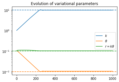
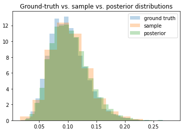
I realized that I could rewrite my problem by rewriting y_{t+1} = (1 + r_t) y_t as r_t = (y_{t+1}/y_t) - 1, and then using that as a direct observation of the distribution for the r’s. Now the variational parameters do converge to their ground truth values, and the distribution matches.

So my model/guide are now

class RegressionModel:
    def __init__(self, mean, std):
        # Convert mean/std into parameters of the gamma dist.
        k = (mean/std)**2
        theta = (std**2)/mean
        self.k = torch.tensor(float(k))
        self.theta = torch.tensor(float(theta))
    
    def model(self, y):
        N = len(y)-1
        k = pyro.param("k", self.k, constraint=tconst.positive)
        theta = pyro.param("theta", self.theta, constraint=tconst.positive)
        with pyro.plate("data", N):
            r = (y[1:]/y[:-1]) - 1
            pyro.sample(f"obs", pdist.Gamma(k, 1/theta), obs=r)
        
    def guide(self, y):
        pass

parameter_evolution

posterior

Thank you for being my rubber duck :slight_smile:

yes deterministic relationships are a bit tricky:

  • either you rewrite your program to get rid of them
  • or you do some analog of your sigma trick. this can work quite poorly though. typically, as sigma goes to zero inference gets harder but as sigma gets large the model is quite different from the one you actually want. this is related to abc

Thank you for the reference, I’ve never heard of abc before, will check it out!

I noticed that there is a pyro.deterministic primitive; would there be any way to use that get around the “rewriting” trick? It’s fairly easy to do in the example I proposed where you can invert to get the sample by itself on the LHS, but what if you have a linear regression model like y = w1*x1 + w2*x2, where the y, x1, x2 are data points and w1, w2 are samples from some distribution? I know in the linear regression tutorial the sigma trick is used… but I believe that only works because the data is actually normally distributed around the regression line and the true model is y = \sum_i w_i*x_i + \epsilon where \epsilon ~ N(0,\sigma). Is there any way to substitute pyro.deterministic for that?

pyro.deterministic can’t really help with inference as such. it’s mostly a way of keeping track of deterministic computations that happen within your program.

it’s precisely in the case where things aren’t analytically invertible that things get tricky.

in the case of linear regression there is no “trick”; the normal prior and normal observation noise are the designed modelling assumptions.

@martinjankowiak I think I figured out a more satisfying resolution that allows me to do what I wanted to do originally (which was infer the distributions of random variables θ from equations like y = f(x,θ) without f necessarily being invertible; in my case f(x,θ)=log(1+θ) + log(x) which is invertible for θ, but the pattern seems easily generalizable to functions that aren’t). The key was to use a combination of TransformedDistributions to model the target variable, and Delta distributions to “sample” the variational parameters. Unfortunately the use of Delta causes the ELBO to be infinite, but hey, I suppose that’s a fair tradeoff for having a functioning model.

Anyway, here’s my new model/guide:

class Model:
    """
    This models the system of equations y_{i+1} = (1+r)*y_i, where r ~ Gamma(k, theta).
    The object is to perform inference and reconstruct the distribution of r using SVI
    (which means recovering the parameters k and theta).
    """
    def __init__(self, k, theta):
        # Specify the parameters of the prior, and also the starting
        # values of the variational parameters
        self.k = torch.tensor(float(k))
        self.theta = torch.tensor(float(theta))
    
    def model(self, y, train=True):
        N = len(y) - 1
        with pyro.plate("data", N):
            # K and theta are variational parameters, but we still need to "sample" them
            k = pyro.sample("k_", Delta(self.k))
            theta = pyro.sample("theta_", Delta(self.theta))
            # Now we need to specify the distribution of the target in terms
            # of transformed distributions
            x = Gamma(k, 1/theta) # The original distribution for r
            x = TransformedDistribution(x, AffineTransform(1., 1.)) # 1+r
            x = TransformedDistribution(x, ExpTransform().inv) # log(1+r)
            X, Y = torch.log(y[:-1]), torch.log(y[1:])
            Yhat = TransformedDistribution(x, AffineTransform(X, 1.)) # log(1+r) + log(y_i)
            obs = pyro.sample("obs", Yhat, obs=Y)
        
    def guide(self, y):
        N = len(y) - 1
        k = pyro.param("k", self.k, constraint=tconst.positive)
        theta = pyro.param("theta", self.theta, constraint=tconst.positive)
        with pyro.plate("data", N):
            # Even though k and theta aren't random variables, we still need
            # to sample them so the guide knows it needs to optimize them
            pyro.sample("k_", Delta(k))
            pyro.sample("theta_", Delta(theta))
            
    def r(self, N=1):
        # Useful for sampling from the posterior of r
        k = pyro.param("k", self.k, constraint=tconst.positive)
        theta = pyro.param("theta", self.theta, constraint=tconst.positive)
        return Gamma(k, 1/theta).sample([N])

I think the use of TransformedDistribution here was critical, as the hack I was using previously of sampling from Normal(Y, 1e-3) isn’t well-founded. Looking back on the first code snippet, it seems like my mistake was trying to first sample from the distribution for r itself, then apply deterministic transformations to the samples, instead transforming then sampling (which seems more natural), as I have done here.

I probably spent 50 hours trying to figure out this simple problem, but I consider it time well spent; I feel like my grasp of Bayesian inference has gone up 10x trying to figure this out! I’m planning to use Pyro more often in the future, seems like a great package!

Also, here’s some visual proof that I did finally solve the problem:

parameter_evolution

distributions