Speed up Numpyro Model

[pankajb64]

I’m seeking advice on improving runtime performance of the below numpyro model.

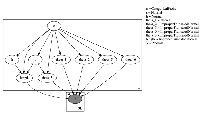
Model Description: I have a dataset of L objects. For each object, I sample a discrete variable c and eight continuous variables – s , h and six parameters theta_i which determine an analytical function (defined by the method dst). This function is fit to observed data points, one fit per object. Ideally the fitting code should be in a nested plate, but since the number of observed data points for each object maybe different, I have instead flattened out all the data points as a single vector V and do the fitting in a separate plate. The total number of data points is SL. The code and graphical model are at the end of this post.

When testing on a dataset of L ~ 3000, SL ~ 21000 , it takes ~ 5 minutes to run 4 chains with 1000 iterations each (500 warmup, 500 sample) on a machine with 8-core CPU and 32 GB ram. However, when testing on a larger dataset of L ~ 3e5 SL ~ 4e6, it takes ~1.5 days.

I am seeking advice on how to speed-up the sampling. I suspect that a large vectors of million data points is causing performance problems for numpyro. Is there any way to tell the sampler to run things in batches of smaller size?

The code. The distribution ImproperTruncatedNormal is just a Normal distribution with positive support as suggested in this thread.

class ImproperTruncatedNormal(dist.Normal):
    support = dist.constraints.positive

funsor.distribution.make_dist(ImproperTruncatedNormal, param_names=("loc", "scale"))

def dst(theta, time):
    return theta[..., 0] + 0.5*theta[..., 1] * (
        jnp.tanh(theta[..., 4] * (time - theta[..., 2])) - 
        jnp.tanh(theta[..., 5] * (time - theta[..., 3]))
    )


def my_model(V_obs, t, index_mapping, L, pi, theta_mean, theta_std, s_line_fit_params, h_line_fit_params, s_prior, h_prior, sigma, SL):
    
    with numpyro.plate("L", L):
        c = numpyro.sample("c", dist.Categorical(jnp.array(pi)), infer={'enumerate': 'parallel'})
        
        s = numpyro.sample("s", dist.Normal(loc=jnp.array(s_prior[c, 0]), scale=jnp.array(s_prior[c, 1])))
        h = numpyro.sample("h", dist.Normal(loc=jnp.array(h_prior[c, 0]), scale=jnp.array(h_prior[c, 1])))
        
        
        theta_1 = numpyro.sample("theta_1", dist.Normal(loc=jnp.array(theta_mean[c, 0]), scale=jnp.array(theta_std[c, 0])))
        theta_2 = numpyro.sample("theta_2", ImproperTruncatedNormal(loc=jnp.array(theta_mean[c, 1]), scale=jnp.array(theta_std[c, 1])))
        theta_5 = numpyro.sample("theta_5", ImproperTruncatedNormal(loc=jnp.array(theta_mean[c, 2]), scale=jnp.array(theta_std[c, 4])))
        theta_6 = numpyro.sample("theta_6", ImproperTruncatedNormal(loc=jnp.array(theta_mean[c, 3]), scale=jnp.array(theta_std[c, 5])))
        
        gamma_3 = jnp.array(s_line_fit_params[c, 0] + s * s_line_fit_params[c, 1])
        gamma_4 = jnp.array(h_line_fit_params[c, 0] + h * h_line_fit_params[c, 1])
        gamma_length = gamma_4 - gamma_3
        sigma_gamma_length = jnp.sqrt(theta_std[c, 3]**2 - theta_std[c, 2]**2)
        
        theta_3 = numpyro.sample("theta_3", ImproperTruncatedNormal(loc=gamma_3, scale=theta_std[c, 2]))
        length = numpyro.sample("length", ImproperTruncatedNormal(loc=gamma_length, scale=sigma_gamma_length))
        theta_4 = numpyro.deterministic("theta_4", theta_3 + length)
        
        theta = numpyro.deterministic("theta", jnp.stack([theta_1, theta_2, theta_3, theta_4, theta_5, theta_6], axis=-1))
        
    with numpyro.plate("SL", SL):
        v_t = dst(theta[..., index_mapping, :], t)
        V = numpyro.sample("V", dist.Normal(v_t, sigma), obs=V_obs)

The graphical model

[fehiepsi]

Hi @pankajb64, it is still a research problem to design algorithms that deal with large datasets. I would suggest using SVI with subsampling rather than MCMC. For MCMC, you might want to try Example: Hamiltonian Monte Carlo with Energy Conserving Subsampling — NumPyro documentation

[pankajb64]

Thanks for sharing that @fehiepsi, I’m trying the HMCECS algorithm for my model but i’m facing issues.
My model has a discrete site c that is to be enumerated over. However, when running SVI, I’m getting an error saying
ValueError: Continuous inference cannot handle discrete sample site 'c'.

I’ve never used SVI before so any advice would be appreciated. Does SVI not work with enumerate discrete variables?

I replaced Trace_ELBO() for the SVI loss with TraceGraph_ELBO, since the documentation suggests that it can deal with discrete latent variables. I’m using AutoGuides for now since I don’t know what guides are and what role they’re supposed to play. I noticed that the documentation says AutoGuides work for continuous variables, so maybe I need to define my own guide?

[fehiepsi]

maybe I need to define my own guide?

Yes. We need a custom guide for TraceGraph_ELBO. Currently, we don’t have support for TraceEnum_ELBO (issue #741), which can work with AutoGuides, yet. Another option is to distribute the likelihood computation into different devices, but it is a pending issue (#1425) - I’m taking a look at it. Sorry, I don’t have better solutions.

[pankajb64]

@fehiepsi Thanks for sharing two issues, I have subscribed to notifications and will keep an eye out for progress.

Before trying to understanding SVI and Guides, I am thinking its worth checking whether it would be faster if I separated the dataset into smaller batches and ran the sampler on each batch in a loop. Something like how its done in this post.

That post mentions how I could speed things up by using jit_model_args=True in that case to avoid recompiling the model for each batch. Each of the L instances in my dataset can be sampled independently, so batching is possible. However the batches will not all be the same shape, since the value of SL will be different. Your comment here mentions how I can still use jit_model_args=True in this case if my model has no local latent variables and I can pad my dataset and use masking. Can you explain what you mean by local latent variables? Does that mean latent variables inside a plate? I’m trying to figure out if my model above has local latent variables and whether the approach I mention here is possible in my case.

[fehiepsi]

I just looked back at your model. We appear to be unable to enumerate it because the variable “V” (which is dependent on “c”) does not belong to the plate “L” (violate restriction 2).

Alternative to jit_model_args=True, you can also do

@jax.jit
def get_samples(batch, key):
    mcmc = MCMC(...)
    mcmc.run(...)
    return mcmc.get_samples(...)

Re local variables: they are latent variables that have the data dimension (i.e., belong to the SL plate in your case).

[pankajb64]

Thanks, I’ll take a look at the @jax.jit mechanism.

Re local latent variables, based on your definition, it doesn’t seem there are any of these in my model. The only variables are theta – which is deterministic, and V, which is observed.

Re the problem with enumeration, I would be interested in knowing if I can reimplement the model to avoid this situation. In principle, the SL plate should be nested within L plate, but from my (limited) understanding of numpyro, that’s not doable.

For each element l in the L plate, I need to estimate a function (parameterized by theta) and fit that function to a certain number of observations v_l, which are observed. v_l is not the same for each l.

Is there a way to get the index of iteration with a plate? If yes, then I could write a code like this.

with numpyro.plate("L", L):
   ...
   theta = ...
        
   l = <get index of iteration>
   v_l_obs = array_of_observations[l]
   t_l = array_of_times[l]
   size_l = v_l.size
   
    with numpyro.plate("SL_nested", size_l):
        v_t = dst(theta, t_l)
        v_l = numpyro.sample("v_l", dist.Normal(v_t, sigma), obs=v_l_obs)

[fehiepsi]

Yes, you can get index using for i in plate(...): but it would make your model very slow to run. For your data size, it is best to use vectorization, rather than for loop.

Looking like the model is your last comment can be enumerated (making sure that your SL_nest plate operates on -2 dimension by specifying dim=-2 in plate statement - it’s best practice to specify dim explicitly). You will need to reshape array_of_observations/times to size_l x L - for this you’ll need masking. It’s better to do it outside of the model to save computations during the model run (inputs of model will be obs, times, mask). After reshaping, you can do inference for each batch (along SL_nested dimension) of (obs, times, mask).

[pankajb64]

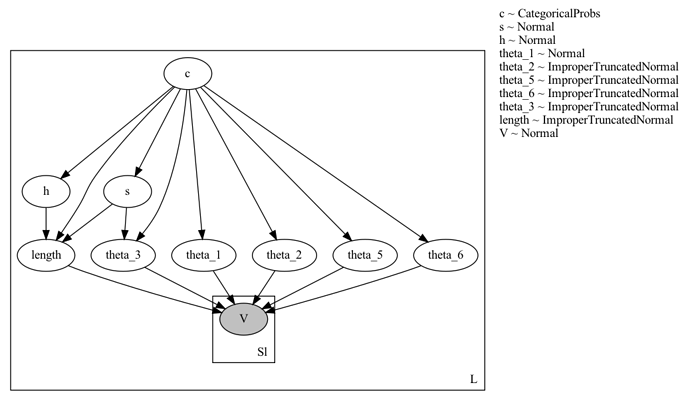
Sorry I’ve been very late to respond. Thanks for this suggestion. I tried this and was able to make the second plate nested using masking. The new model looks like this.

def my_model(data, times, data_mask, L, pi, theta_mean, theta_std, s_line_fit_params, h_line_fit_params, s_prior, h_prior, sigma, Sl):
    
    with numpyro.plate("L", L):
        c = numpyro.sample("c", dist.Categorical(jnp.array(pi)), infer={'enumerate': 'parallel'})
        
        s = numpyro.sample("s", dist.Normal(loc=jnp.array(s_prior[c, 0]), scale=jnp.array(s_prior[c, 1])))
        h = numpyro.sample("h", dist.Normal(loc=jnp.array(h_prior[c, 0]), scale=jnp.array(h_prior[c, 1])))
        
        
        theta_1 = numpyro.sample("theta_1", dist.Normal(loc=jnp.array(theta_mean[c, 0]), scale=jnp.array(theta_std[c, 0])))
        theta_2 = numpyro.sample("theta_2", ImproperTruncatedNormal(loc=jnp.array(theta_mean[c, 1]), scale=jnp.array(theta_std[c, 1])))
        theta_5 = numpyro.sample("theta_5", ImproperTruncatedNormal(loc=jnp.array(theta_mean[c, 2]), scale=jnp.array(theta_std[c, 4])))
        theta_6 = numpyro.sample("theta_6", ImproperTruncatedNormal(loc=jnp.array(theta_mean[c, 3]), scale=jnp.array(theta_std[c, 5])))
        
        gamma_3 = jnp.array(s_line_fit_params[c, 0] + s * s_line_fit_params[c, 1])
        gamma_4 = jnp.array(h_line_fit_params[c, 0] + h * h_line_fit_params[c, 1])
        gamma_length = gamma_4 - gamma_3
        sigma_gamma_length = jnp.sqrt(theta_std[c, 3]**2 - theta_std[c, 2]**2)
        
        theta_3 = numpyro.sample("theta_3", ImproperTruncatedNormal(loc=gamma_3, scale=theta_std[c, 2]))
        length = numpyro.sample("length", ImproperTruncatedNormal(loc=gamma_length, scale=sigma_gamma_length))
        theta_4 = numpyro.deterministic("theta_4", theta_3 + length)
        
        theta = numpyro.deterministic("theta", jnp.stack([theta_1, theta_2, theta_3, theta_4, theta_5, theta_6], axis=-1))
        
        with numpyro.plate("Sl", Sl, dim=-2):
            with numpyro.handlers.mask(mask=data_mask):
                v_t = dst(theta, times)
                V = numpyro.sample("V", dist.Normal(v_t, sigma), obs=data)

Graphically it looks like this

[pankajb64]

When testing this new model, it seems that the predictions for continuous variables s and h are mostly identical to the old model, but the predictions for the discrete variable c are often different – on average the precision/recall metrics for the discrete variable are worse in the new model.

I noticed another puzzling thing. The way I’m testing these models is by splitting the dataset into smaller batches of L ~ 4000 each and running the models independently on each batch – the approach I mentioned in post #5 above. It seemed that for some batches, the new model would sample much faster (15s vs 500s for the old model) but produce really bad predictions – all the samples for s and h are the same as the initial value provided. And for the batches where it produces good predictions, it takes longer to run than the old model.

So in short, this change slows the model down, causes it to generally predict worse on the discrete variable, and occasionally causes it to predict complete trash.

This is when sampling only with HMC. I’m guessing that if I add SVI, I could make the model faster, but from what I understand SVI would not help solve the issue of worse precision/recall metrics? Any other ideas/suggestions would also be appreciated.