There are a few things going on. First, your model is rigid because you enforce that the standard deviation of the response variable must be equal to 1. Second, I am not sure why you would place the mean of the prior on the bias to the mean of the design variable – this means that your prior assumptions are that the mean of the response variable is equal to the mean of the design variable, and I’m not sure why that would be the case. Third, you did not standardize your model inputs. Contrary to popular opinion that does not automatically place you in a state of sin, but it does move you closer – particularly in your case, since you have enforced that sigma = 1 and thus you will not be able to account for much noise in the (unnormalized) response variable.
I think that maybe you are trying to replicate cell 13 in the ipynb that you linked. Unfortunately there are some not-so-great things going on there as well. In particular, there is a hypothesis that the standard deviation is a uniform distribution between zero and some multiple of the standard deviation of the response. It is usually inadvisable to put a uniform prior on a scale parameter because, in doing so, you are saying that there is literally no possibility that the scale parameter can be larger than the upper value of the uniform. Of course, that is not true.
Here is an alternate ols model that seems to get the job done:
brainvolcc = torch.tensor(
    [438., 452., 612., 521., 752., 871., 1350.],
    dtype=torch.float
)
masskg = torch.tensor(
    [37.0, 35.5, 34.5, 41.5, 55.5, 61.0, 53.5],
    dtype=torch.float
)

# standardize the rvs
norm_brain = (brainvolcc - brainvolcc.mean()) / brainvolcc.std()
norm_mass = (masskg - masskg.mean()) / masskg.std()


def ols(X, y=None):
    assert len(X.shape) <= 2
    if len(X.shape) < 2:
        X = X.unsqueeze(-1)

    intercept = pyro.sample(
        'intercept',
        dist.Normal(0.0, 1.0)
    )
    beta = pyro.sample(
        'beta',
        dist.Normal(0, 1.0).expand((X.shape[-1],))
    )

    mu = pyro.deterministic('mu', X.matmul(beta) + intercept)

    sigma = pyro.sample('sigma', dist.LogNormal(0., 1.))
    response = pyro.sample(
        'response',
        dist.Normal(mu, sigma),
        obs=y
    )
    return mu
I fit it the same way you do: using AutoDiagonalNormal and using the Adam optimizer:
guide = pyro.infer.autoguide.AutoDiagonalNormal(ols)
optim = pyro.optim.Adam({'lr': 0.01})
svi = pyro.infer.SVI(ols, guide, optim, loss=pyro.infer.Trace_ELBO())

pyro.clear_param_store()
niter = 2500

for n in range(niter):
    loss = svi.step(norm_mass, y=norm_brain)
    if n % 250 == 0:
        print(f"On iteration {n}, loss = {loss}")
My loss starts at around 20 and decreases to a plateau around 10 or so.
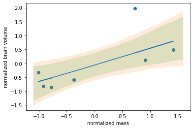
The effects of a) data normalization and b) allowing the standard deviation to take on a sane range of values leads us to a decent data fit:
posterior_predictive = pyro.infer.Predictive(
    ols,
    guide=guide,
    num_samples=1000
)
posterior_samples = posterior_predictive(norm_mass, y=norm_brain)

fig, ax = plt.subplots()

ax.scatter(norm_mass, norm_brain)
ax.plot(
    norm_mass,
    posterior_samples['mu'].median(dim=0)[0].detach()
)

linspace = torch.linspace(-1.1, 1.6, 100)
ellipse_samples = posterior_predictive(linspace)
reg_lines_quantiles = pyro.ops.stats.quantile(
    ellipse_samples['mu'].detach(),
    [0.05, 0.1, 0.9, 0.95]
)
for i in range(2):
    ax.fill_between(
        linspace,
        reg_lines_quantiles[i],
        reg_lines_quantiles[-(i + 1)],
        alpha=0.15
    )
The resulting regression line ellipses: