Fitting a model with a multimodal posterior using flows and NeuTra HMC

[fbartolic]

Hi!

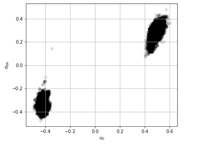
I decided to try out Pyro/Numpyro to test the latest normalizing flow algorithms on my astrophysics model. The model is simple, consisting of only 7 parameters, but the posterior is usually multimodal (in a predictable way).

Here’s an outline of the model

def model(t, F, Ferr):
    ln_DeltaF = numpyro.sample("ln_DeltaF", dist.Normal(4., 4.))
    DeltaF = jnp.exp(ln_DeltaF)
    ln_Fbase = numpyro.sample("ln_Fbase", dist.Normal(2., 4.))
    Fbase = jnp.exp(ln_Fbase)
    t0 = numpyro.sample("t0", dist.Normal(ca.utils.estimate_t0(event), 20.))
    ln_tE = numpyro.sample("ln_tE", dist.Normal(3., 6.))
    tE = jnp.exp(ln_tE)
    u0 = numpyro.sample("u0", dist.Normal(0., 1.))
    piEE = numpyro.sample("piEE", dist.Normal(0., .5))
    piEN = numpyro.sample("piEN", dist.Normal(0., .5))

    # Trajectory
    zeta_e_t = jnp.interp(t, points, zeta_e)
    zeta_n_t = jnp.interp(t, points, zeta_n)
    zeta_e_t0 = jnp.interp(t0, points, zeta_e)
    zeta_n_t0 = jnp.interp(t0, points, zeta_n)
    zeta_e_dot_t0 = jnp.interp(t0, points, zeta_e_dot)
    zeta_n_dot_t0 = jnp.interp(t0, points, zeta_n_dot)

    delta_zeta_e = zeta_e_t - zeta_e_t0 - (t - t0) * zeta_e_dot_t0
    delta_zeta_n = zeta_n_t - zeta_n_t0 - (t - t0) * zeta_n_dot_t0

    u_per = u0 + piEN * delta_zeta_e - piEE * delta_zeta_n
    u_par = (
        (t - t0) / tE + piEE * delta_zeta_e + piEN * delta_zeta_n
    )
    u = jnp.sqrt(u_per**2 + u_par**2)
    
    # Magnification
    A_u = (u ** 2 + 2) / (u * jnp.sqrt(u ** 2 + 4))
    A_u0 = (u0 ** 2 + 2) / (jnp.abs(u0) * jnp.sqrt(u0 ** 2 + 4))
    A = (A_u - 1) / (A_u0 - 1)

    # Predicted flux
    F_pred = DeltaF*A + Fbase
    
    ln_c = numpyro.sample("ln_c", dist.Exponential(1/2.))
    
    numpyro.sample("data_dist", dist.Normal(F_pred, jnp.exp(ln_c) * Ferr), obs=F)

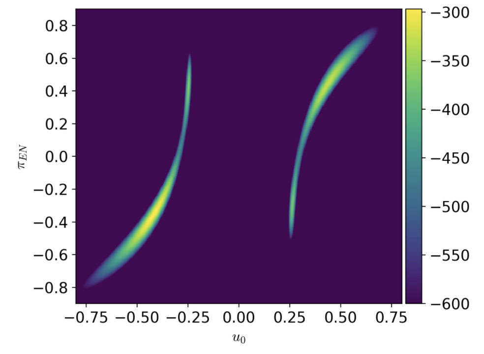
When I sample the model with NUTS the sampler finds only one of the modes because the posterior is multimodal in the u_0 parameter. Here’s what the likelihood surface looks like when evaluated on a (u0, piEN) grid while keeping all the other parameters fixed:

Ideally, I’d like to be able to train a guide which finds both modes and pass the guide to HMC for use in NeuTra HMC.

Based on this example, I thought the AutoBNAFNormal autoguide might be able to catch both modes, however, after testing various combinations of input parameters I find that it always gets stuck in one of the modes. Even when I fix all of the parameters and fit for the parameters in a 2D subspace of the full parameter space, it fails to find both modes except for a few very particular combinations of the learning rate and input parameters to AutoBNAFNormal.

My questions are the following:

• Is there a better choice for a guide which would work well for this kind of problem?
• I’ve read a paper tackling a similar problem where they used a 20 block MAF and a mixture of Gaussians for the base distribution of the flow and they seem to be able to recover multiple modes. How can I implement this in Pyro? Can I change the base distribution for AutoBNAFNormal? I’ve read the docs on constructing custom guides but I don’t really know where to start.

Thanks!

[fehiepsi]

This is interesting. I think AutoBNAF can do the job if you make it sophisticated enough (by changing num_flows and hidden_factors in the constructor).

Can I change the base distribution for AutoBNAFNormal ?

The AutoBNAFNormal implementation is actually simple (it just requires a few lines of code) and you can change the base distribution by inherit it and change the get_base_dist method. If you want to use mixture of Gaussians as base distribution then it is better to use Pyro (mainly because MCMC might not work well with mixture of normals).

I will take a closer look this weekend if you can provide some synthesis data.

Is there a better choice for a guide which would work well for this kind of problem?

There are many new normalization flows in Pyro that you can try. @stefanwebb wrote this great tutorial, which you can start with.

[fbartolic]

I tried changing the AutoBNAF parameters and still I get only one of the modes.

The AutoBNAFNormal implementation is actually simple (it just requires a few lines of code) and you can change the base distribution by inherit it and change the get_base_dist method. If you want to use mixture of Gaussians as base distribution then it is better to use Pyro (mainly because MCMC might not work well with mixture of normals).

Thanks, I’ll try this out!

I will take a closer look this weekend if you can provide some synthesis data.

Here is a reproducible example:

GitHub - fbartolic/pyro_flows

I’d be curious to see if you can make it work. There are lots of problems in astronomy with similar structure and It’d be really exciting if we could use NUTS for those.

[fehiepsi]

Thanks, @fbartolic! It is interesting to see that you are using many features that NumPyro supports. I have played with your notebooks a bit and faced the same problem as you. We have some discussions about multimodal in this thread, there Joshua implemented nested sampling to deal with the multimodal issue. It can be a good method to try on your problem.

This is the first time I face this problem, so I hope there will be more interesting discussions looking forward, especially from ones who read this thread and have some experiences dealing with this issue. Here are things I have tried

Convert the model to a mixture model

def model(...):
    ...
    K = 2  # 3, 4
    p = numpyro.sample("probs", dist.Dirichlet(jnp.ones(K)))
    c = numpyro.sample("cluster", dist.Categorical(probs=p))
    with numpyro.plate("num_clusters", K):
        u0 = numpyro.sample("u0", dist.Normal(0.0, 1.0))[c]
        piEE = numpyro.sample("piEE", dist.Normal(0.0, 0.5))[c]
        piEN = numpyro.sample("piEN", dist.Normal(0.0, 0.5))[c]
    ...
    with numpyro.plate("data", len(F)):
        return numpyro.sample("data_dist", ...)

init_vals["u0"] = jnp.array([-0.5, 0.5])  # not set initial u0 value

but the mixture only concentrates on 1 mode (even when I enable x64 mode numpyro.enable_x64())…

Run multi-chain mcmc

• As you observed, with different seeds, we get different samples. You can set num_chains=10, chain_method="vectorized" if your CPU does not have enough cores to run parallel chains. Or if you have GPU, you can set a much higher num_chains with the hope that the sampling is still fast enough and there is no memory issue happen…
• This approach looks most promising to me. However, I am not sure what is a good method to combine those chains. I found this paper: Adaptive MCMC via Combining Local Samplers but the algorithm is a bit complicated.

If you know a good approach, please open an FR in github so we can try to implement it.

Use MixtureNormal as base_dist

• I followed your suggestion and used mixture normal as base_dist, but the issue still happens.

from numpyro.contrib.tfp import distributions as tfd

class AutoBNAFMixture(AutoBNAFNormal):
    def get_base_dist(self):
        C = 10  # the number of mixtures
        mixture = tfd.MixtureSameFamily(tfd.Categorical(probs=jnp.ones(C) / C),
                                        tfd.Normal(jnp.arange(float(C)), 0.1))
        return mixture.expand([self.latent_dim]).to_event()

• I also changed the activation function from Tanh to ELU or LeakyReLU (defined below) but the issue still happens.

def LeakyReLU():
    def init_fun(rng, input_shape):
        return input_shape, ()

    def apply_fun(params, inputs, **kwargs):
        x, logdet = inputs
        out = nn.leaky_relu(x)
        t_logdet = jnp.where(x >= 0, 0, jnp.log(0.01))
        return out, logdet + t_logdet.reshape(logdet.shape[:-2] + (1, logdet.shape[-1]))

    return init_fun, apply_fun


def ELU():
    def init_fun(rng, input_shape):
        return input_shape, ()

    def apply_fun(params, inputs, **kwargs):
        x, logdet = inputs
        out = nn.elu(x)
        t_logdet = -nn.relu(-x)
        return out, logdet + t_logdet.reshape(logdet.shape[:-2] + (1, logdet.shape[-1]))

    return init_fun, apply_fun

There are lots of problems in astronomy with similar structure

Interesting! May I ask which methods astronomers use to overcome the issue?

[fbartolic]

Thank you so much for the super detailed response!

We have some discussions about multimodal in this thread, there Joshua implemented nested sampling to deal with the multimodal issue. It can be a good method to try on your problem.

Nested sampling does work well for this problem. The issue I had with it in the past is that it is many orders of magnitude slower than HMC. This JAX implementation looks really promising and it might turn out to be very efficient. I’ll definitely try it out. The issue with NS in general is that it doesn’t scale well to high dimensions (above ~30) and while it does an OK job at exploring the bulk of the modes, I found that the ESS for tails of the posterior is pretty bad.

Run multi-chain mcmc

• As you observed, with different seeds, we get different samples. You can set num_chains=10, chain_method="vectorized" if your CPU does not have enough cores to run parallel chains. Or if you have GPU, you can set a much higher num_chains with the hope that the sampling is still fast enough and there is no memory issue happen…
• This approach looks most promising to me. However, I am not sure what is a good method to combine those chains. I found this paper: Adaptive MCMC via Combining Local Samplers but the algorithm is a bit complicated.

Thanks for the reference, that looks interesting. I came across saw this recent paper on stacking chains from multiple runs which looks interesting and it the method looks like it’s lot easier to implement. I’ll try it out and report what I find!

Use MixtureNormal as base_dist

• I followed your suggestion and used mixture normal as base_dist, but the issue still happens.

I find the same thing. Here is the paper I mentioned which uses MAF on a similar multimodal problem. Here’s what they say in the paper:

Each block of the MAF (which is a “MADE” [5]) adapts a fixed ordering of the dimensions and applies
affine transformations iteratively for each dimension, subject to the autoregressive condition. We
adopt random orderings for each of the 20 block to maximize network expressibility. As binary
microlensing often exhibit degenerate, multi-modal solutions, we use a mixture of eight Gaussians
for each dimension of the base distribution

It’s a slightly different problem from the one we’re discussing here because they they are doing likelihood free inference but they seem to be able to model the multimodal structure with a set of MAFs and a large mixture of Gaussians for the base distribution. I might try recreating their approach at some point but there’s no hope of using Neutra HMC in this case because the base distribution is multimodal.

Interesting! May I ask which methods astronomers use to overcome the issue?

In my subfield they do a grid search for the modes on a 2D subspace of the entire parameter space and report some summary statistics for each. Nested sampling has been really popular and also rejection sampling for low dimensional problems.

[joshuaalbert]

@fehiepsi Thanks for the tag. This is exactly the problem I faced with a multimodal posterior from an astronomical problem. @fbartolic I’d be happy if you wanted to use jaxns. I am actively developing it, and it’s very promising. It’s about 3 orders of magnitude faster that polychord, multinest and dynesty. And it’ll only get faster as I improve the code. I have a bunch of examples in the repo that should get you started, however feel free to post a question on the issues if you’re having trouble. Maybe start with this example: https://github.com/Joshuaalbert/jaxns/blob/master/jaxns/examples/jones_scalar_data_tec_prior.py

[fehiepsi]

@fbartolic I just made a wrapper for @joshuaalbert’s jaxns at this PR. Could you take a look and let me know if the result here is expected? Nested sampling seems to capture multi-modal posterior. (I don’t have any background on nested sampling so I didn’t change any of its parameters - probably you can get better results by changing some of them. In particular, I am not sure why its performance seems good but effective sample size is small…)

[joshuaalbert]

It looks good. Once you address the resampling remark I made under the PR the ESS will be correct, as well as the statistics.

This integration also makes me want to fully document the jaxns code, so thank you for this motivation!

[fehiepsi]

@joshuaalbert I tried to compare NUTS vs NS in that PR’s notebook. It seems to me that NUTS outperforms NS in the above model+data. With default parameters, maximum log likelihood of NS is -2164 while most MCMC samples have log likelihoods around -1378. I think having some guidelines to use NS effectively would be very helpful.

[joshuaalbert]

@fehiepsi, yes I think I could provide some guidelines.
These are the nested sampling args:

num_live_points: ~(D+1) * (# modes in posterior) * 50
max_samples: ~few * num_live points * information_gain (information gain is roughly how many e-folds of prior space need to be covered before getting to bulk of the posterior), in your example notebook information_gain=-H=53.3, so maybe use 2*53.3*num_live_points
collect_samples: True only if you want to collect samples (which you do in this case)
termination_frac: 0.001 to 0.01 is fine
stoachastic_uncertainty: leave this false for your purposes
sampler_kwargs: dict(
    depth:int, This says how many clusters to maintain. JAX NS can handle 2^(depth-1) posterior modes, You can over specify. Maybe 3-5 is robust to most moderately complex cases, 
    num_slices:int how many iterations of slice sampling to do per NS step. Probably 1 or 2 is enough. In some cases, raising this to 2 or 3 with get better results.)

Note that by only computing the maximum likelihood like this max(ns._results.log_L_samples[:65854]) that you’ll miss any samples beyond 65854 and in NS the likelihood samples are ordered from smallest to largest. If NS is not converging then likely you’re not giving it enough max_samples or termination fraction should be lower. Notice that in your diagnostic plot (3rd row) it starts to turn up at the end, this implies that the sampling was not done.

[fehiepsi]

Awesome, thanks! I got pretty good result for the above model with num_live_points=2000, max_samples=2e5, sampler_kwargs=dict(depth=5, num_slices=3).

[fbartolic]

Wow jaxns is looking really good, I tested NUTS, dynesty (a popular NS package) and jaxns on this problem. I used similar settings for dynesty and jaxns and the results all match:

The difference in runtime between dynesty and jaxns is huge, ~2min vs ~48min on my Macbook! @joshuaalbert do you have a sense of where this massive speedup is coming from? dynesty is written in pure Python so it makes sense that it’s slower but I wouldn’t expect a big difference between polychord/multinest and jaxns running on a CPU.

[joshuaalbert]

@fbartolic thanks! The timing of 2min probably also includes the compile time, so if you neglect that it’s even faster! I think the difference in speed is because the whole algorithm is jit-compiled with XLA, which can bring significant speed ups. Indeed, jaxns even seems to be orders of magnitude faster than polychord and multinest. Another example where XLA makes a huge difference is BFGS. It’s much faster than scipy+numpy or even when combining scipy+jax.

[fbartolic]

Run multi-chain mcmc

• As you observed, with different seeds, we get different samples. You can set num_chains=10, chain_method="vectorized" if your CPU does not have enough cores to run parallel chains. Or if you have GPU, you can set a much higher num_chains with the hope that the sampling is still fast enough and there is no memory issue happen…
• This approach looks most promising to me. However, I am not sure what is a good method to combine those chains. I found this paper: Adaptive MCMC via Combining Local Samplers but the algorithm is a bit complicated.

If you know a good approach, please open an FR in github so we can try to implement it.

@fehiepsi, I tried the approach from Yao et.al. 2020 (see also Yao et.al. 2018). I run 4 HMC chains initialized such that each one ends up in in one of 4 modes shown in the likelihood plot I posted earlier. There are two dominant posterior modes comparable in posterior mass and two less significant modes. I compute two kinds of weights described in the paper, the pseudo-BMA+ weights and the “stacking” weights. As I understand it, Pseudo-BMA+ should give something close to the full Bayesian posterior except more robust to changes in the data. With stacking, the goal is to jointly optimize the weights for all chains such that the predictive performance of a linear combination of all models (modes) is maximized. Here are the results and the notebook for reproducing all the plots:

If you look at loo values, it seems that all 4 modes have very similar cross validation performance with the first two modes being slightly better. The pseudo-BMA+ weights give non-negligible weights for modes 3 but the stacking weights are noticeably different. Mode 4 gets a zero weight, presumably because its cross validation performance is identical to mode 3 so it doesn’t improve the predictive performance of the linear sum of all modes. This plot shows the stacked posterior for the u0 parameter:

The colored histograms are the 4 HMC chains, the dashed histogram is the true Bayesian posterior we get with jaxns (assuming it’s working correctly) and the solid histogram is the stacked posterior which is generally different from the Bayesian posterior.

I’m liking this approach and I’m not even sure I want the true posterior anymore because the true posterior assigns insignificant weights to the inner two modes (red and green) and it’s not clear to me that it’s closer to truth than the stacked posterior. In the stacked posterior the only physical parameter I really care about in this model, tE, has a very different distribution with a heavy tail towards large values so it matters a great deal whether you’re discarding the inner two modes or not.

I also like this approach because it can easily be automated by running lots of parallel chains and stacking them after inference. One thing I haven’t figured is how to run a large number of chains in parallel, on a GPU, I set

numpyro.util.set_platform('gpu')
numpyro.util.set_host_device_count(50)

And run HMC with num_chains=50 but I get the following error:

/usr/local/lib/python3.6/dist-packages/numpyro/infer/mcmc.py:428: UserWarning: There are not enough devices to run parallel chains: expected 50 but got 1. Chains will be drawn sequentially. If you are running MCMC in CPU, consider to use `numpyro.set_host_device_count(50)` at the beginning of your program.
  .format(self.num_chains, xla_bridge.device_count(), self.num_chains))

@fehiepsi do you know what’s going on here?

[fehiepsi]

Oh, I have seen this type of stacking previously to compare models but didn’t notice that we can use this to weight chains too. Thanks for pointing it out, @fbartolic!! In case it is helpful, ArviZ has a utility compare which can compute the model weights for you. It would be really nice if we can put those infos in a tutorial.

how to run a large number of chains in parallel, on a GPU

This is not supported in JAX (host devices are CPU devices). You need to use multiple GPUs to achieve this. If you want to collect a lot of chains, then either running in CPUs or setting chain_method="vectorized" (probably with a smaller max_tree_depth < 10 because in vectorized method, every chains have to wait, for all chains finishing their current sample step, before going the the next sample step).

[fbartolic]

This is not supported in JAX (host devices are CPU devices). You need to use multiple GPUs to achieve this. If you want to collect a lot of chains, then either running in CPUs or setting chain_method="vectorized" (probably with a smaller max_tree_depth < 10 because in vectorized method, every chains have to wait, for all chains finishing their current sample step, before going the the next sample step).

@fehiepsi so when they run thousands of chains in parallel in the NeuTra HMC paper with the Tensorflow NUTS implementation, this is equivalent to chain_method="vectorized" in numpyro?

Also, is there a way to have a different starting point for each chain using the init_to_value initialization startegy without creating a new MCMC object for each chain?

[fehiepsi]

It is quite similar but not the same. The paper uses a fixed step size and number of leapfrog steps for each chain. To achive that, you can put mcmc run under jax vmap transform

def get_samples(step_size, num_leapfrog_steps):
    kernel = HMC(model, step_size=step_size, adapt_step_size=False, trajectory_length=step_size * num_leapfrog_steps)
    mcmc = MCMC(kernel, 1000, 1000)
    mcmc.run(...)
    return mcmc.get_samples()

samples = vmap(get_samples)(batch_of_stepsizes, batch_of_numsteps)

You might also want to disable adapt mass matrix and set num warmup to 0.

This also applies for your second question, in case you also want to have different step sizes, mass matrices across mcmc runs (which is more suitable to the stacking method in your comment). Here we can use pmap instead of vmap.

If you want to use a single MCMC run with different initial values, then you can do it through init_params (uncontrained values of samples) argument in mcmc.run but you need to set initial values for all parameters. I guess it is tricky to make init_to_value works for a batch of initial constrained values but if you want, please open a FR on github.

[joshuaalbert]

@fbartolic in order to be sure that jaxns is giving correct results, can you share the settings you used? You can also just share the code, and I can inspect.

[fbartolic]

Here you go:

Here are the results and the notebook for reproducing all the plots:

[joshuaalbert]

@fbartolic, it looks good, but try setting depth=1. While counter intuitive, depth=1 can ensure that all the posterior modes are caught, however efficiency can suffer. Next jaxns release will have big improvements to this aspect of performance. Also, make sure that the samples_jaxns are being resampled by @fehiepsi’s wrapper. His initial code forgot to resample, but then he added resampling, so you may need to repull that branch. If it’s not resampled then the histograms don’t make sense.