Discrete Inference with TraceGraph_ELBO

Hi all,

I’ve been testing the new TraceGraph_ELBO implementation in numpyro for a sparse regression model and haven’t been able to get reasonable results. I’m unsure if this is due to variance in the gradients or if there is an aspect I am still missing.

The model I’ve implemented is the Sum of Single Effects model (ie SuSiE; see here). Even in a relatively low dimension (n = 400 and p = 10) the model seems unable to identify the variables with nonzero effect. I’ve provided the numpyro implementation alongside a simple implementation of the IBSS approach described in the above paper here.

Here is my model and guide:

# define the model
def model(X, y, l_dim) -> None:

    n_dim, p_dim = jnp.shape(X)

    # fixed prior prob for now
    logits = jnp.ones(p_dim)
    beta_prior_log_std = softplus_inv(jnp.ones(l_dim))
    with numpyro.plate("susie_plate", l_dim):
        gamma = numpyro.sample("gamma", dist.Multinomial(logits=logits))
        beta_l = numpyro.sample("beta_l", dist.Normal(0.0, nn.softplus(beta_prior_log_std)))

    # compose the categorical with sampled effects
    beta = numpyro.deterministic("beta", beta_l @ gamma)
    loc = X @ beta
    std = numpyro.param("std", 0.5, constraint=constraints.positive)
    with numpyro.plate("N", n_dim):
        numpyro.sample("obs", dist.Normal(loc, std), obs=y)

    return


def guide(X, y, l_dim) -> None:

    n_dim, p_dim = jnp.shape(X)

    # posterior for gamma
    g_shape = (l_dim, p_dim)
    gamma_logits = numpyro.param("gamma_post_logit", jnp.ones(g_shape))

    # posterior for betas
    b_shape = (p_dim, l_dim)
    b_loc = numpyro.param("beta_loc", jnp.zeros(b_shape))
    b_log_std = numpyro.param("beta_log_std", softplus_inv(jnp.ones(b_shape)))
    with numpyro.plate("susie_plate", l_dim):
        gamma = numpyro.sample("gamma", dist.Multinomial(logits=gamma_logits))

        # average across individual posterior estimates
        post_mu = numpyro.deterministic("post_mu", jnp.sum(gamma.T * b_loc, axis=0))
        post_std = numpyro.deterministic("post_std", jnp.sum(gamma.T * nn.softplus(b_log_std), axis=0))
        beta_l = numpyro.sample("beta_l", dist.Normal(post_mu, post_std))

    return

And inference is being performed as:

scheduler = exponential_decay(args.learning_rate, 5000, 0.9)
adam = optim.Adam(scheduler)
svi = SVI(model, guide, adam, TraceGraph_ELBO())

# run inference
results = svi.run(
    rng_key_run,
    args.epochs,
    X=X,
    y=y,
    l_dim=args.l_dim,
    progress_bar=True,
    stable_update=True,
)

The numpyro model results in a completely flat posterior and is unable to select the relevant variables, whereas the simple IBSS CAVI-style approach has no such troubles. I’ve tried different learning rates and decay with no luck. Similarly, increasing the number of particles didn’t seem to help much, which would suggest that variance in gradients isn’t necessarily the issue. Is there some other aspect I’m missing with the TraceGraph_ELBO capabilities?

EDIT: I updated the guide to explicitly average over individual posteriors and see improved performance, but not quite at what IBSS can capture.

EDIT2: Here is are renderings of the model and guide:
susie.model
susie.guide

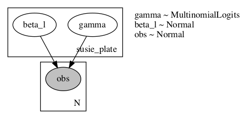
Given the explicit computation of beta_l moments from gamma I would have expected an arrow indicating the dependency in the posterior beta_l <- gamma, but I’m unsure if this is a result of the plate setup, or how rendering works when given a guide.

Could you try to set num_particles to 1000 to have a lower variance?

@nmancuso the achilles heel of variational inference is discrete latent variables. basically because they don’t play nice with gradients. in particular the gradient variance can be very very high (for discussion see here).

if i understand your model correctly the graphical model structure is such that you are going to be in the regime of high variance. this is basically because the gamma variables have a large “downstream cost”, in particular resulting from the likelihood term.

this isn’t necessarily very easy to address within the context of stochastic variational inference. one route is to increase num_particles until the variance becomes manageable. another is to use a fancier gradient estimator, e.g. use “baselines” as is possible in pyro (but not afaik currently in numpyro). but even these tricks may not be enough. this is presumably why susie doesn’t use stochastic variational inference.

stochastic variational inference is nice because it’s “black-box”. but for the same reason it can catastrophically fail in some classes of models.

1 Like

@nmancuso can you also explain what’s going on here? it seems that you’re breaking the rules of plates.

Thanks, @fehiepsi and @martinjankowiak.

This seems to work in the low dimensional setting (p_dim = 10), but begins to fail in more realistic settings (for my use case) of p_dim = 1000 when n_dim = 400. I had tried increasing the number of particles earlier, but not to this extent and my worry is that this may depend on some exponential number of samples between p_dim and num_particles to handle the combinatorial nature of the problem.

This code is selecting which of the beta mean/std parameters to select for the posterior based on gamma for each l_dim. I reparameterized the guide in terms of parameters wrt each data variable (p_dim) and then select each for l_dim using the sampled gamma vector. Indexing would be a bit cleaner, but I ran into JIT errors and just used this product/sum solution which does the same thing.

Using a bit more formal notation, let \text{beta_loc}_{pl} := \mathbb{E}[b_l | \gamma_{lp} = 1, X, y] be the conditional posterior expectation of b_l given that it is coupled with the p th column of X. Since \sum_p \gamma_{lp} = 1 for fixed l, the code jnp.sum(gamma.T * beta_loc, axis=0) selects the posterior means for each b_l by setting it to the corresponding \text{beta_loc}_{pl} values.

I had an earlier implementation that skipped this step and directly parameterized the l_dim normal space, but its poor performance led me to try this option. In hindsight, in the CAVI solution, the posterior parameters for beta_l depend on gamma, by ‘selecting’ which variable to use for the posterior mean/std, so trying to back out conditional posteriors from each beta_l shouldn’t work, hence the above formulation.

My understanding of the above plate implementation is that variables are conditionally independent along the l_dim, but not necessarily the other dimensions (here, each of the l beta_l values). Is that correct?

Thanks again for your input.

@nmancuso unfortunately for all practical purposes i think it’s essentially impossible to get SVI to work in these kinds of models, especially if you want to push to large p. for moderate p (say p<50) you could do gibbs updates w.r.t. the discrete latent variables and use HMCGibbs (so you’d be doing HMC w.r.t. continuous latent variables).

if you want to use SVI you need to relax the discrete latent variables to continuous latent variables, e.g. by using a horseshoe prior or some other shrinkage prior.

if you want discrete latent variables i suggest this approach, although this is obviously a fair bit of effort to code up. (i intend to open source an implementation of this algorithm at some point, but i don’t know how long that will take me…; the author also links to an R implementation)

what’s your real goal?

1 Like