Hi, I am stuck with a seemingly simple problem. I have a mathematical model composed of various non-linear sums of gaussian distributions (x1, x2, x3, x4).
y = A*x1 + B*(torch.exp(-x2 / C)) + C*x3 + torch.log10(x4)
x1 and x2 are known variables, x3 and x4 have gaussian distribution with a fixed mean and std. I am using the simulated y as my observations and trying to infer the distribution of the latent variables x3 and x4.
Unfortunately, I am not able to infer the distribution of the ground truth. ELBO doesn’t seem to be maximizing no matter what I try. I tried different learning rates, changed the mean and std of the latent variables in the model and guide to be close to the true values, but it seems to do a random walk around the parameters I have specified in the model and fail to converge. I also tried using AutoDiagonalNormal, it seems to do a little better, but the posterior values seem to converge to some local minima far from my ground truth.
I must be doing something horribly wrong. If the only way for me to infer the latent variable is by known the prior to be very close to the truth, then I could simply use my model and try varying the unknown parameters until it matches with the distribution. My current code isn’t even able to get me to the ballpark.
I would appreciate if you could suggest ways to make the model robust and help with optimal strategy to select the model parameters.
## Define the mathematical model
def model(y,x1,x2):
x3 = pyro.sample("x3", dist.Normal(200, 100))
x4 = pyro.sample("x4", dist.Normal(120, 90))
# Use the mathematical model to compute the expected output
expected_output = A*x1 + B*(torch.exp(-x2 / C)) + C*x3 + torch.log10(x4)
# Likelihood of the observed output
pyro.sample("y", dist.Normal(expected_output, 20.0), obs=y)
## Define the updated guide with Normal distributions for x3 and x4
def guide(y,x1,x2):
x3_mean_guide = 150.0
x3_std_guide = 10.0
x4_mean_guide = 120.0
x4_std_guide = 25.0
# Sample x3 and x4 from the guide as Normal
x3 = pyro.sample("x3", dist.Normal(x3_mean_guide, x3_std_guide))
x4 = pyro.sample("x4", dist.Normal(x4_mean_guide, x4_std_guide))
return {"x3": x3, "x4": x4}
## Generate synthetic data
A = 50.0
B = 150.
C = 2.0
D = 10.0
### Specify known information about x1 and x2 (mean and std deviation)
x1_mean = 60.0
x1_stddev = 5.0
x2_mean = 10.0
x2_stddev = 2.0
x3_mean_true = 180.0
x3_stddev_true = 5.0
x4_mean_true = 80.0
x4_stddev_true = 25.0
x1 = pyro.sample("x1", dist.Normal(x1_mean, x1_stddev))
x2 = pyro.sample("x2", dist.Normal(x2_mean, x2_stddev))
## Simulated data
true_x3 = dist.Normal(x3_mean_true, x3_stddev_true).sample((200,))
true_x4 = dist.Normal(x4_mean_true, x4_stddev_true).sample((200,))
observed_output = A*x1 + B*(torch.exp(-x2 / C)) + C*true_x3 + torch.log10(true_x4)
## Setup SVI for variational inference
pyro.clear_param_store()
#guide = AutoDiagonalNormal(model)
adam_params = {"lr": .01, "betas": (0.95, 0.999)}
optimizer = Adam(adam_params)
svi = SVI(model, guide, optimizer, loss=TraceGraph_ELBO())
elbo_values = [ ]
num_steps = 30
for step in range(num_steps):
loss = 0
for val in observed_output:
loss += svi.step(val, x1, x2)
elbo_values.append(-loss / len(observed_output))
print(step, loss)
## Extract the learned distribution of x3 and x4 from the guide
samples = [ ]
num_samples = 500
for _ in range(num_samples):
posterior = guide(observed_output,x1,x2)
x3_sample = posterior["x3"].item()
x4_sample = posterior["x4"].item()
samples.append((x3_sample, x4_sample))
## Print the mean and standard deviation of the inferred distributions
x3_samples = [x[0] for x in samples]
x4_samples = [x[1] for x in samples]
print("x3 mean:", torch.mean(torch.tensor(x3_samples)))
print("x3 std dev:", torch.std(torch.tensor(x3_samples)))
print("x4 mean:", torch.mean(torch.tensor(x4_samples)))
print("x4 std dev:", torch.std(torch.tensor(x4_samples)))
## Visualize the Data
### Convert true values to numpy arrays
true_x3_value = true_x3.numpy()
true_x4_value = true_x4.numpy()
predicted_output=A*x1 + B*(torch.exp(-x2 / C)) + C*torch.tensor(x3_samples) + torch.log10(torch.tensor(x4_samples))
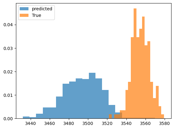
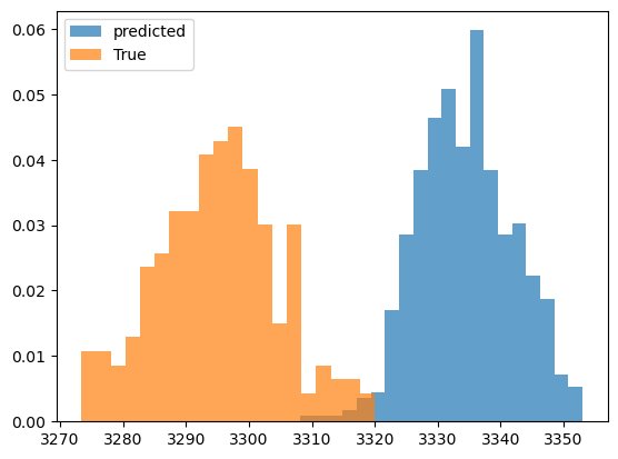
plt.figure()
plt.hist(predicted_output.detach().numpy(), bins=20,alpha=0.7,label='predicted',density=True)
plt.hist(observed_output.detach().numpy(), bins=20,alpha=0.7,label='True',density=True)
plt.legend()
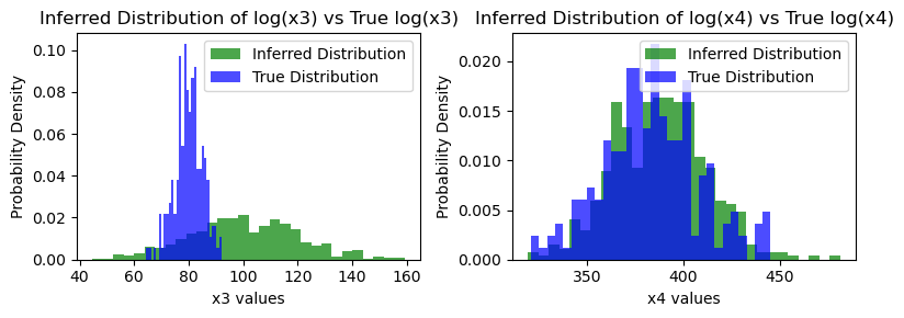
### Visualize the true values vs the inferred distributions
plt.figure(figsize=(12, 4))
plt.subplot(1, 2, 1)
plt.hist(x3_samples, bins=30, density=True, alpha=0.7, color='green', label='Inferred Distribution')
plt.hist(true_x3.detach().numpy(), bins=30, density=True, alpha=0.7, color='blue', label='True Distribution')
plt.xlabel('x3 values')
plt.ylabel('Probability Density')
plt.legend()
plt.subplot(1, 2, 2)
plt.hist(x4_samples, bins=30, density=True, alpha=0.7, color='green', label='Inferred Distribution')
plt.hist(true_x4.detach().numpy(), bins=30, density=True, alpha=0.7, color='blue', label='True Distribution')
plt.title('Inferred Distribution of log(x4) vs True log(x4)')
plt.xlabel('x4 values')
plt.ylabel('Probability Density')
plt.legend()
plt.tight_layout()
plt.show()
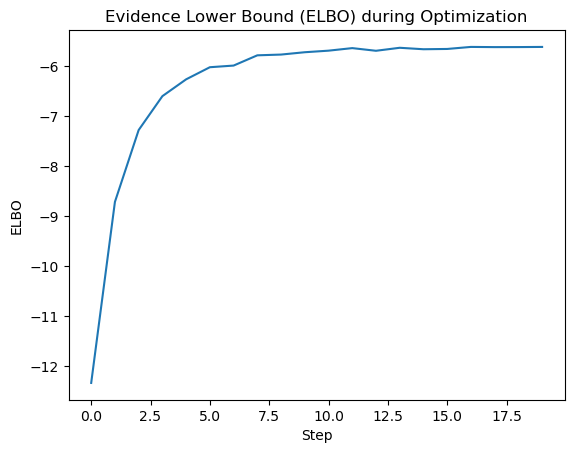
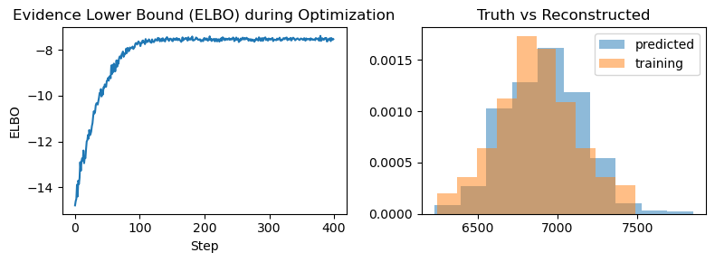
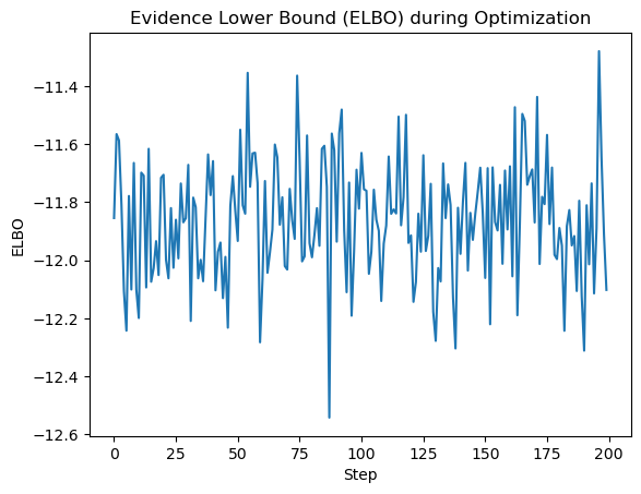
# Plot the ELBO values
plt.plot(elbo_values)
plt.xlabel('Step')
plt.ylabel('ELBO')
plt.title('Evidence Lower Bound (ELBO) during Optimization')
plt.show()
Here is the ELBO
Inferred vs Truth Latent Variables:

Inferred vs Truth Output Variables: