UPDATE: I figured out the problem and fixed it. It was as simple as moving w_loc, w_log_sig, b_loc, b_log_sig inside the for loop. My understanding is that each dataset requires different random initializations. I compared both performance and coefficients/intercepts with sklearn and they are very close.
Original post below.
Hi, I am implementing a VBLR model in Pyro and had a question on Pyro’s output.
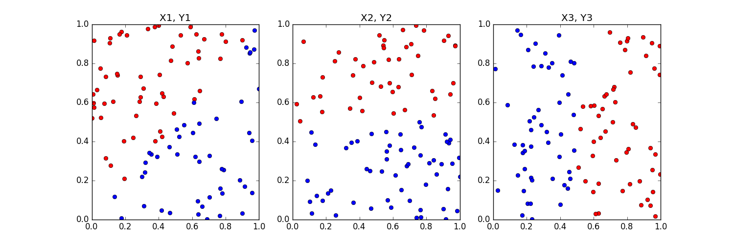
To make the problem concrete, assume you have three datasets of the form {X1, Y1}, {X2, Y2} and {X3, Y3}. Here X’s is a N x p matrices and Y’s are N x 1 binary vector of labels, N = 100 and p = 2 for all datasets with equal proportion of positive and negative labels per dataset. See sample plot below for an idea of the datasets.
I get valid weights and bias term when training one VBLR model per dataset i.e. setup Model, Guide and use SVI. Pretty Straightforward.
Now, I would like to learn the weights for the three datasets simultaneously. When doing so I get identical weights and bias term for ALL three datasets. I am not sure what I am doing incorrectly here.
Learning the weights and bias terms simultaneously is, in my mind, implementing the plate notation in the graphical model below,
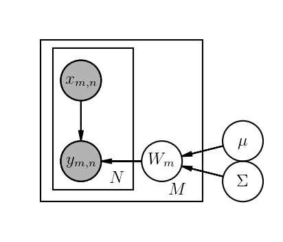
Here M = 3 and N = 100. The \mu and \Sigma are fixed priors over weights.
Below is my code for Model, Guide and Bayesian logistic regression when M = 3. I implement Bayesian logistic regression as a one layer neural network with Sigmoid activation. Below M is represented via vector tasks as [0,…,0, 1,…,1, 2,…,2].
# NN with one Sigmoid layer
class neural_network_model(nn.Module):
	def __init__(self, p):
		super(neural_network_model, self).__init__()
		self.linear = nn.Linear(p, 1)
		self.non_linear = nn.Sigmoid()

	def forward(self, x):
		return self.non_linear(self.linear(x))

p = 2 # number of features
nn_model = neural_network_model(p)

def model(X, Y, tasks):
	N, p = X.size()
	M = len(tasks.unique())
	for m in pyro.irange("task_loop", M):
		# Create unit normal priors over the parameters
		loc = torch.zeros(1, p)
		scale = 2 * torch.ones(1, p)
		w_prior = dist.Normal(loc, scale)

		bias_loc = torch.zeros(1)
		bias_scale = 2 * torch.ones(1)
		b_prior = dist.Normal(bias_loc, bias_scale)

		priors = {"linear.weight": w_prior, "linear.bias": b_prior}

		# lift module parameters to random variables sampled from the priors
		lifted_module = pyro.random_module("module_{}".format(m), nn_model, priors)

		# sample a neural network (which also samples w and b)
		lifted_reg_model = lifted_module()

		prediction_mean = lifted_reg_model(X[torch.ByteTensor(tasks == m), :].float()).squeeze(-1)

		pyro.sample("obs_{}".format(m), dist.Bernoulli(prediction_mean), obs=Y[torch.ByteTensor(tasks == m)])

def guide(X, Y, tasks):
	N, p = X.size()
	M = len(tasks.unique())
	softplus = nn.Softplus()

	# Create unit normal priors over the parameters
	w_loc = torch.randn(1, p)
	w_log_sig = -3.0 * torch.ones(1, p) + 0.05 * torch.randn(1, p)
	b_loc = torch.randn(1)
	b_log_sig = -3.0 * torch.ones(1) + 0.05 * torch.randn(1)

	module_list = []
	for m in pyro.irange("task_loop", M):
		# register learnable params in the param store
		mw_param = pyro.param("guide_mean_weight_{}".format(m), w_loc)
		sw_param = softplus(pyro.param("guide_log_scale_weight_{}".format(m), w_log_sig))
		mb_param = pyro.param("guide_mean_bias_{}".format(m), b_loc)
		sb_param = softplus(pyro.param("guide_log_scale_bias_{}".format(m), b_log_sig))

		# gaussian guide distributions for w and b
		w_dist = dist.Normal(mw_param, sw_param).independent(1)
		b_dist = dist.Normal(mb_param, sb_param).independent(1)

		dists = {"linear.weight": w_dist, "linear.bias": b_dist}

		# lift module parameters to random variables sampled from the priors
		lifted_module = pyro.random_module("module_{}".format(m), nn_model, dists)

		# sample a neural network
		module_list.append(lifted_module())

	return module_list
When running this code and printing out the parameters I get,
[guide_mean_weight_0]: tensor([[ 0.2431, 3.2466]])
[guide_mean_weight_1]: tensor([[ 0.2431, 3.2466]])
[guide_mean_weight_2]: tensor([[ 0.2431, 3.2466]])
When running this code separately on each dataset I get,
[guide_mean_weight_0]: tensor([[ -4.82, 4.59]])
[guide_mean_weight_1]: tensor([[ -1.43, 5.57]])
[guide_mean_weight_2]: tensor([[ 6.43, -0.75]])
guide_mean_bias_0: tensor([ 0.1174])
guide_mean_bias_1: tensor([-0.0226])
guide_mean_bias_2: tensor([-2.8482])
In both cases, I executed SVI for 10K iterations with learning rate 0.001. You can assume all random seeds are fixed so that results are reproducible.
Why are the VBLR coefficients identical in the former case?