I am currently trying to leverage DKL according to (Example: Deep Kernel Learning — Pyro Tutorials 1.8.4 documentation) in an active learning scenario. The task I am working on is a binary classification task therefore I am also using the Binary likelihood as specified in the tutorial. This all works pretty OK and the classifier is learning.
Since in an active learning scenario I need to add more and more data points to the training set, I would like to use the model to drive the decision which training point to add next. Therefore I use the model to make a prediction on the remaining data points and then select the datapoint where the model is most insecure (has the highest variance). Now as it seems the Binary likelihood I use returns a vector of zeros and ones when calling Binary(some_vector). What I need though is a full fledged Bernoulli distribution which gives me a mean and variance for each of my remaining data points. To make that happen, this is the prediction method I came up with:
 with torch.no_grad():
     for data, target in data_loader:
         if self.cuda:
             data, target = data.cuda(), target.cuda()
         target = target.float()

         # get prediction of GP model on data
         f_loc, f_var = self.gpmodule(data)

         # convert f_loc and f_var into bernoulli distribution
         # this I copied from the forward method of the Binary likelihood
         f = torch.sigmoid(dist.Normal(f_loc, f_var.sqrt())())
         y_dist = dist.Bernoulli(f) # this I copied from the forward method of the Binary likelihood
         pred = self.gpmodule.likelihood(f_loc, f_var)
         # I return the Bernoulli distribution the targets and the predictions from calling the Binary likelihood
         return y_dist, target, pred
This gives me the desired distribution for all my remaining datapoints y_dist. Now I use y_dist to get the mean (y_dist.mean), the variance (y_dist.variance) and if I need to the binary predictions y_dist.mean.ge(0.5).
Somehow I think this is doing the trick, but since I am new to this game and framework, I am not entirely sure if this is how its done. Maybe someone a little more experienced can take a short look and tell me if I’m doing it right or if I messed up big time!
I think that to get mean and variance of f, you can take 100 samples of dist.Normal(f_loc, f_var.sqrt()), apply sigmoid, and take the mean and variance of these samples. It is more reasonable to me than take 1 sample of f and compute mean/variance based only on that single sample.
Ah OK. It also felt like something was wrong here. So to get the correct mean and variance I have two versions of the prediction code
Version 1
        with torch.no_grad():
            for data, target in data_loader:
                if self.cuda:
                    data, target = data.cuda(), target.cuda()
                target = target.float()

                # get prediction of GP model on data
                f_loc, f_var = self.gpmodule(data)
                pred = self.gpmodule.likelihood(f_loc, f_var)

                # draw 300 predictions (samples) from Normal
                predictions = []
                for i in range(300):
                    predictions.append(torch.sigmoid(dist.Normal(f_loc, f_var.sqrt())()))
                predictions = torch.stack(predictions)

                # calculate mean and variance of the 300 predictions
                mean = torch.mean(predictions, dim=0)
                var = torch.var(predictions, dim=0)

                return mean, var, target, pred
This version aims to implement your suggestion, if I understood it correctly.
Version 2
        with torch.no_grad():
            for data, target in data_loader:
                if self.cuda:
                    data, target = data.cuda(), target.cuda()
                target = target.float()

                # get prediction of GP model on data
                f_loc, f_var = self.gpmodule(data)
                pred = self.gpmodule.likelihood(f_loc, f_var)

                # draw 300 predictions (samples) from Normal
                prediction = []
                for i in range(300):
                    prediction.append(torch.sigmoid(dist.Normal(f_loc, f_var.sqrt())()))
                prediction = torch.stack(prediction)

                # pass predictions through Bernoulli distribution
                y_dist = dist.Bernoulli(prediction)

                # compute the average mean and variance for all samples
                mean = torch.mean(y_dist.mean, dim=0)
                var = torch.mean(y_dist.variance, dim=0)

                return mean, var, target, pred
This version passes the predictions through a dist.Bernoulli distribution before computing the average mean and var over all 300 prediction samples.
I’m not sure whether it’s even allowed to pass the predictions through the Bernoulli and calculate the mean of all the returned mean and variance values?
What do you think? Which one is the valid approach?
Hi @milost, I think dist.Bernoulli(prediction).mean is just the same as prediction, so I guess two approaches will give similar results for mean. About var, it depends on what is your definition of it. If you want to compute the variance of prob predictions, then the first approach is valid. If you want to compute the variance (I guess it is harder to interpret this notion because Bernoulli is a discrete distribution) of pred, then you can replace the second approach by calling self.gpmodule.likelihood(f_loc, f_var) 300 times and taking mean/variance of the preds.
OK, so what you are suggesting for the second approach should turn out to be:
with torch.no_grad():
    for data, target in data_loader:
        if self.cuda:
            data, target = data.cuda(), target.cuda()
        target = target.float()

        # get prediction of GP model on data
        f_loc, f_var = self.gpmodule(data)

        # draw 300 predictions (samples) from likelihood
        predictions = []
        for i in range(300):
            predictions.append(self.gpmodule.likelihood(f_loc, f_var))
        predictions = torch.stack(predictions)

        # compute the mean and variance for the drawn prediction samples
        mean = torch.mean(predictions, dim=0)
        var = torch.var(predictions, dim=0)

        return mean, var, target, mean.ge(0.5)
This should then be the “correct” process for the second version.
I’ll give both versions a try and see which one works better in steering the selection strategy in an active learning setting. If its of any interest I will report back which one worked better for me.
As promised, I report back with two results of my experiments with both prediction methods in my active learning setting.
I have increasingly expanded the training set to include the elements for which the current trained model was most uncertain (maximum uncertainty). I have expanded the training set up to a maximum of 20 percent of the total training data and recorded Precision, Recall and F1 when predicting on the entire training dataset. So basically the experiments tries to answer the question … If I show you an increasing amount of training examples how much of the total training set are you going to predict correctly? (Or put it differently with how little training data can I get away with when trying to predict on the entire dataset)
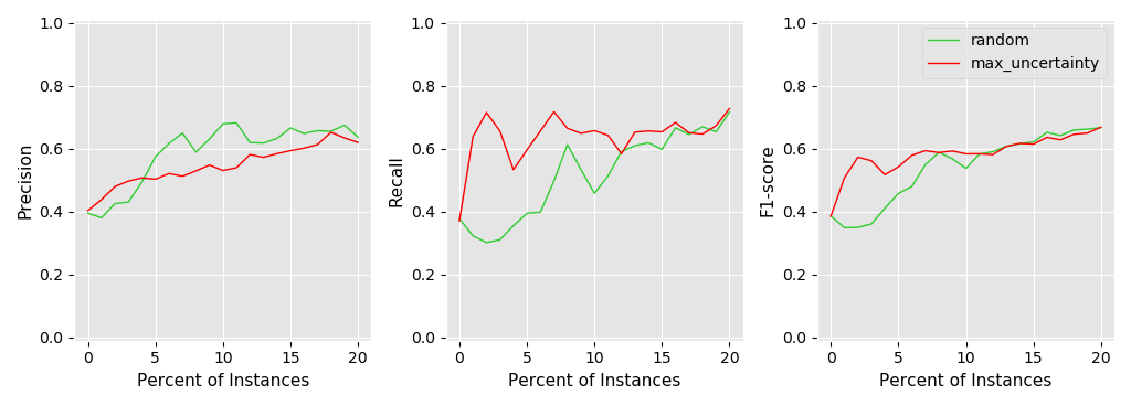
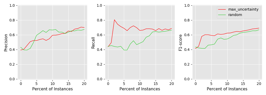
Now without further ado … here are the plots. First for Version 1 of the prediction method, followed by Version 2 of the prediction method:
As both plots show, using maximum uncertainty is able to reach an overall classification F1 of 0.6 much faster then using a random selection strategy. So for example in Version 2 the maximum uncertainty strategy is able to reach an F1 of 0.6 using only between 3-4% of the training data while using a random selection strategy the model needs to be exposed to something between 13-14% of the data in order to reach the same F1.
So I guess both prediction methods do the job while the Version 2 seems to be somewhat smoother but this could very well be due to optimizer behaviour. This experiments have at max an indicative nature since they are only run on one of my datasets. Should anyone be interested in this feel free to PM me.
Last but not least again a big THANK YOU @fehiepsi who helped me a lot to handle the DKL and was really responsive!! You are definitely in my book of cool ppl