Hi @ALund. I’ll share a few things and try to clarify some points.
What your model (or the segment of it that you’ve provided does) is a little nonstandard (not that there’s anything wrong with that):
- it posits that there’s a single latent 2d path that evolves for
data.shape[0] - 1 timesteps
- There are
N noisy observations of this single path (that’s your plate and y stuff)
In addition there’s an error with your initialization of data_plate; if you try running that, you’ll get
TypeError: arange() received an invalid combination of arguments - got (torch.Size, device=torch.device), but expected one of:
 * (Number end, *, Tensor out, torch.dtype dtype, torch.layout layout, torch.device device, bool pin_memory, bool requires_grad)
 * (Number start, Number end, Number step, *, Tensor out, torch.dtype dtype, torch.layout layout, torch.device device, bool pin_memory, bool requires_grad)
since plate wants a single positive integer telling it how many terms in the product there are.
I think that what your model may have been intended to do (and many apologies if you did truly mean the interpretation above!) is the more conventional N observations of timeseries of length T. These timeseries of length T correspond to latent rvs (your x_1 and x_2 above) and observed noisy realizations y.
Here’s a little model that does exactly that. It’s in 1d and models just a latent random walk and centered state space uncertainty. But it should be pretty clear how you can modify it to meet your needs!
def state_space_model(data, N=1, T=2, prior_drift=0., verbose=False):
    # global rvs
    drift = pyro.sample('drift', dist.Normal(prior_drift, 1))
    vol = pyro.sample('vol', dist.LogNormal(0, 1))
    uncert = pyro.sample('uncert', dist.LogNormal(-5, 1))

    if verbose:
        print(
            f"Using drift = {drift}, vol = {vol}, uncert = {uncert}"
        )

    # the latent time series you want to infer
    # since you want to output this, we initialize a vector where you'll
    # save the inferred values
    latent = torch.empty((T, N))

    # I think you want to plate out the same state space model for N different obs
    with pyro.plate('data_plate', N) as n:
        x0 = pyro.sample('x0', dist.Normal(drift, vol))  # or whatever your IC might be
        latent[0, n] = x0

        # now comes the markov part, as you correctly noted
        for t in pyro.markov(range(1, T)):
            x_t = pyro.sample(
                f"x_{t}",
                dist.Normal(latent[t - 1, n] + drift, vol)
            )
            y_t = pyro.sample(
                f"y_{t}",
                dist.Normal(x_t, uncert),
                obs=data[t - 1, n] if data is not None else None
            )
            latent[t, n] = x_t

    return pyro.deterministic('latent', latent)
A few things to note here.
- We write
data[t - 1, n]. This is not because we are being acausal but rather because data should be of shape (N, T - 1). So the t - 1-th element of data should correspond with the t-th element of the latent time series. This is because the latent time series must be one element longer as the Markov assumption depends on an initial condition.
- If our goal were actually to infer latent random walks, this is by far not the most efficient way to implement it.
pyro.markov is fundamentally sequential and thus slow. since a random walk with drift mu and volatility sigma is a deterministic transformation of white noise, something much quicker would be
noise = pyro.sample('noise', dist.Normal(0, 1).expand((T, N)))
random_walk = pyro.deterministic('random_walk', (mu + sigma * noise).cumsum(dim=0))
But this is not what your model does, so I have implemented it using markov to make it easier for you to change to meet your needs!
- We wrapped the tensor of all the latent rvs in a
deterministic so that we can grab it upon model return. This just makes life easier and doesn’t affect the joint density of the model at all.
- Because our
drift, vol, and uncert are global rvs, each run of the model generates substantially different-looking sample paths. Check it out:
    # draws from the prior predictive are shape (T, N)
    # each draw uses different draws from global drift and vol params
    n_prior_draws = 5
    prior_predictive = torch.stack(
        [state_space_model(None, N=N, T=T) for _ in range(n_prior_draws)]
    )

    colors = plt.get_cmap('cividis', n_prior_draws)
    fig, ax = plt.subplots()
    list(map(
        lambda i: ax.plot(prior_predictive[i], color=colors(i)),
        range(prior_predictive.shape[0])
    ))
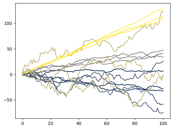
Each color corresponds with a different draw from the prior predictive. We drew 5 different draws, each with N = 3 and T = 100.
Now, to your question about fitting these models. Since we have a random variable x_t for each t in question, it really is not such a bad idea to use one of the built-in autoguides to construct your guide:
    guide = pyro.infer.autoguide.AutoDiagonalNormal(state_space_model)
    optim = pyro.optim.Adam({'lr': 0.01})
    svi = pyro.infer.SVI(state_space_model, guide, optim, loss=pyro.infer.Trace_ELBO())

    niter = 2500  # or whatever, you'll have to play with this and other optim params
    pyro.clear_param_store()
    losses = torch.empty((niter,))

    for n in range(niter):
        loss = svi.step(data, N=data_N, T=data_T)
        losses[n] = loss

        if n % 50 == 0:
            print(f"On iteration {n}, loss = {loss}")
I will say that I do this all the time and it works quite well.
About sampling from the posterior: no problem. There is a great utility class for this called pyro.infer.Predictive:
# you can extract the latent time series in a variety of ways
    # one of these is the pyro.infer.Predictive class
    num_samples = 100
    posterior_predictive = pyro.infer.Predictive(
        state_space_model,
        guide=guide,
        num_samples=num_samples
    )
    posterior_draws = posterior_predictive(None, N=data_N, T=data_T)

    # since our model returns the latent, we should have this in the `latent` value
    print(
        posterior_draws['latent'].squeeze().shape == (num_samples, data_T, data_N)
    )
So that is just about all there is that. Hopefully this is at least somewhat helpful. Feel free to reach out if you have any more questions.