I have a model that has a large number of parameters where most of them are independent, with a subset of them having covariances. I would like to use an AutoMultivariateNormal for the parameters I know to be correlated (approx 8 parameters) and an AutoDiagonalNormal (or AutoLowRankMultivariateNormal, approx 10,000 parameters) for the remaining parameters. What is the best way to go about this in Numpyro? Is there an easy way to mix multiple AutoGuides?
2 Likes
in pyro this can be done pretty easily using block and AutoGuideList but i don’t think this has been implemented in numpyro.
@fehiepsi are there any good workarounds?
I guess we need to use
def indep_model():
    ...

def dep_model():
    ...

indep_guide = AutoDiagonalNormal(indep_model)
dep_guide = AutoMultivariateNormal(dep_model)

def model():
    indep_model()
    dep_model()

def guide():
    indep_guide()
    dep_guide()
It is great to have AutoGuideList.
1 Like
Breaking up the model seems like a good idea, although I am unsure how to go about it in my case.
-
[a, b, c, lam1, lam2]are the variables with potential covariance -
hyper_modelis a function that takes the hyper parameterslam1andlam2and turns them into the width of thexprior -
xis an NxN pixel grid of independent variables (N is ~100) -
simulate_modelis a forward-modelling function that takes in[a, b, c, x]and produces a pixel array of data and noise values to be compared to observations
The goal is to have AutoDiagonalNormal on x and AutoMultivariateNormal on [a, b, c, lam1, lam2]
def full_model(data, N):
    a = numpyro.sample('a', ...)
    b = numpyro.sample('b', ...)
    c = numpyro.sample('c', ...)

    lam1 = numpyro.sample('lam1', ...)
    lam2 = numpyro.sample('lam2', ...)
    simga = hyper_model(lam1, lam2)
    with numpyro.plate('y axis', N):
        with numpyro.plate('x axis', N):
            x = numpyro.sample('x', dist.Normal(0, sigma))

    modeled_data, modeled_noise = simulate_model(a, b, c, x)
    with numpyro.plate('obs y axis', data.shape[0]):
        with numpyro.plate('obs x axis', data.shape[1]):
            numpyro.sample('observed', dist.Normal(modeled_data, modeled_noise), obs=data)
My model is a bit more complicated than this, my x values are actually the 2D FFT of the pixel grid that is passed into simulate_model. I am modelling the pixel grid as coming from a stationary Gaussian Process, so the FFT values are independent and uncorrelated with a width determined by the power spectrum (the hyper_model function in this case).
To break this up would I just do:
def indep_model(N, lam1, lam2):
    simga = hyper_model(lam1, lam2)
    with numpyro.plate('y axis', N):
        with numpyro.plate('x axis', N):
            x = numpyro.sample('x', dist.Normal(0, sigma))
    return x

def dep_model():
    a = numpyro.sample('a', ...)
    b = numpyro.sample('b', ...)
    c = numpyro.sample('c', ...)
    lam1 = numpyro.sample('lam1', ...)
    lam2 = numpyro.sample('lam2', ...)
    return a, b, c, lam1, lam2

indep_guide = AutoDiagonalNormal(indep_model)
dep_guide = AutoMultivariateNormal(dep_model)

def model(data, N):
    a, b, c, lam1, lam2 = dep_model()
    x = indep_model(N, lam1, lam2)
    modeled_data, modeled_noise = simulate_model(a, b, c, x)
    with numpyro.plate('obs y axis', data.shape[0]):
        with numpyro.plate('obs x axis', data.shape[1]):
            numpyro.sample('observed', dist.Normal(modeled_data, modeled_noise), obs=data)

def guide(data, N):
    a, b, c, lam1, lam2 = dep_guide()
    x = indep_guide(N, lam1, lam2)
    <not sure what goes here>
I am assuming something else needs to go in the guide function, but I am not exactly sure what… Also can return statements like these be used inside models and AutoGuides to pass samples from one into another?
2 Likes
Since I am trying to do something similar right now, I tried to get @fehiepsi’s suggestion to work for a simple test case; this is what I came up with so far:
Import statements
import numpyro
import numpyro.distributions as dist
from numpyro.infer.autoguide import AutoNormal, AutoMultivariateNormal, Trace_ELBO
from numpyro import sample, plate
from numpyro.infer import SVI, Predictive, NUTS, MCMC
from numpyro.optim import Adam
from jax import random
import pandas as pd
import seaborn as sns
import numpy as np
import warnings
Model and guide
def params_model(a_loc=None, b_loc=None):
    if a_loc is None:
        a_loc = sample("a_loc", dist.Normal(loc=0.0, scale=4.0))
    if b_loc is None:
        b_loc = sample("b_loc", dist.Normal(loc=0.0, scale=4.0))
    return a_loc, b_loc

def sample_model(a_loc, b_loc, y=None):

    if y is None:
        nobs = 1
    else:
        nobs = len(y)

    with plate("N", nobs):
        lat_a = sample("lat_a", dist.Normal(loc=np.ones((nobs,)) * a_loc, scale=0.1))  # unobserved
        lat_b = sample("lat_b", dist.Normal(loc=np.ones((nobs,)) * b_loc, scale=0.1))  # unobserved
        label = sample("label", dist.Bernoulli(logits=lat_a+lat_b), obs=y)

def model(a_loc=None, b_loc=None, y=None):

    a_loc, b_loc = params_model(a_loc, b_loc)
    sample_model(a_loc, b_loc, y)

params_guide = AutoMultivariateNormal(params_model)
sample_guide = AutoNormal(sample_model)

def guide(y=None):
    params = params_guide()
    sample_guide(params['a_loc'], params['b_loc'], y)
Sampling from the model with specific params for a_loc and b_loc
data = Predictive(lambda **kwargs: model(a_loc=-1, b_loc=2), num_samples=10000)(random.PRNGKey(1))
Inferring a_loc and b_loc from the simulated data using SVI
 # note the small LR and 50k epochs - the model seems to have converged by the end
optimizer = Adam(step_size=0.0001)
svi = SVI(model, guide, optimizer, loss=Trace_ELBO())
svi_result = svi.run(random.PRNGKey(0), 50000, y=data["label"].squeeze())
which produces the following result:
SVI results plotting
svi_predictive = Predictive(guide, params=svi_result.params, num_samples=1000)
svi_samples = svi_predictive(random.PRNGKey(1))
df = pd.DataFrame({'a_loc': svi_samples['a_loc'], 'b_loc': svi_samples['b_loc']})
with warnings.catch_warnings():
    warnings.simplefilter(action='ignore', category=FutureWarning)  # there is an annoying FutureWarning
    sns.pairplot(df)
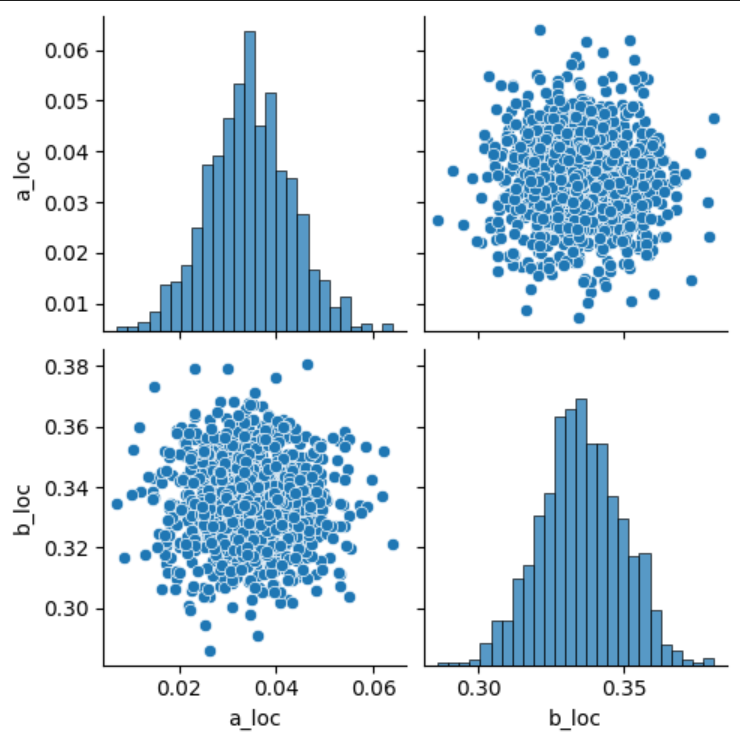
Numerically, we get (from svi_result.params):
'auto_loc': Array([0.03441792, 0.33475387], dtype=float32),
'auto_scale_tril': Array([[8.2799597e-03, 0.0000000e+00],
        [5.1299034e-05, 1.4457051e-02]], dtype=float32)
which seems to agree with the above plots: essentially no correlation is identified between the two parameters. (Assuming I can interpret auto_scale_tril as something like the square root of a covariance matrix?
This was confusing me a bit: I designed the model such that a_loc and b_loc can be trivially and fully traded off against each other, so I would have expected to see much stronger correlation between the two variables. I tried to verify my assumptions using MCMC/NUTS, and that is indeed able to recover the correlation between the two parameters correctly:
MCMC code
nuts_kernel = NUTS(model)
mcmc = MCMC(nuts_kernel, num_samples=1000, num_chains=4, num_warmup=500)
mcmc.run(random.PRNGKey(0), y=data["label"].squeeze())
df_mcmc = pd.DataFrame({'a_loc': mcmc.get_samples()['a_loc'], 'b_loc': mcmc.get_samples()['b_loc']})
with warnings.catch_warnings():
    warnings.simplefilter(action='ignore', category=FutureWarning)  # there is an annoying FutureWarning
    sns.pairplot(df_mcmc)
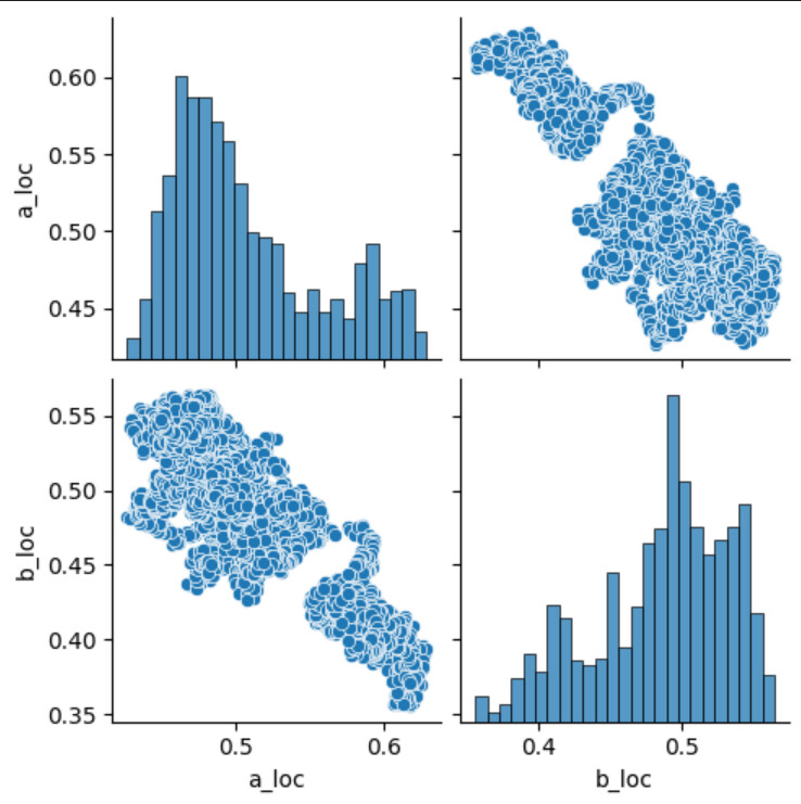
Which leads me to ask: did I do something wrong in the SVI implementation, or in its evaluation?
I ended with a similar implementation for my model. I want to model an image under the prior that the image comes from a power spectrum with a given functional form. Under this model the power spectrum parameters are expected to be correlated, but the pixels in the image will be independent (i.e. any correlation comes from the power spectrum prior only).
Here is the split model using two guides:
# Power spectrum params, assumed to have covariance
def prior_corr(): #, n_prior, s_prior, r_prior):
    n = numpyro.sample('n', dist.HalfCauchy(0.5))
    sigma = numpyro.sample('sigma', dist.HalfCauchy(0.5))
    rho = numpyro.sample('rho', dist.HalfCauchy(150))
    return n, sigma, rho


# Pixel values, assumed to be mostly independent
def prior_pix(n, sigma, rho, shape):
    # a helper function that returns the power spectrum for the 2D Matern kernel
    helper = MaternHelper2D(n, sigma, rho, shape, scale=1)
    # The real and imag parts of the data's FFT are independent normal distributions
    # with scale set by the power spectrum
    scale = jnp.sqrt(helper.P_rk)
    with numpyro.plate(f'pixels plate 1 - {scale.shape[1]}', scale.shape[1]):
        with numpyro.plate(f'pixels plate 2 - {scale.shape[0]}', scale.shape[0]):
            pixels_real = numpyro.sample('pixels_real', dist.Normal(0, scale))
            pixels_imag = numpyro.sample('pixels_imag', dist.Normal(0, scale))
    return pixels_real, pixels_imag


# Full model
def model(data, shape, exposure_time):
    n, sigma, rho = prior_corr()
    pixels_real, pixels_imag = prior_pix(n, sigma, rho, shape)
    source = numpyro.deterministic(
        f'source',
        jnp.fft.irfft2((pixels_real + 1j * pixels_imag), norm='ortho')
    )
    noise_sigma = jnp.sqrt(sigma_bkd**2 + (source / exposure_time))
    with numpyro.plate(f'data 1 - {data.shape[1]}', data.shape[1]):
        with numpyro.plate(f'data 2 - {data.shape[0]}', data.shape[0]):
            numpyro.sample('obs', dist.Normal(source, noise_sigma), obs=data)
For the guides, I want to use an AutoBNAFNormal for the power spectrum params and AutoDiagonalNormal for the image pixels.
init_fun = infer.init_to_median()
# use `prefix` to avoid overlapping names in the multiple guides
dep_guide = autoguide.AutoBNAFNormal(prior_corr, prefix='auto_dep', init_loc_fn=init_fun, hidden_factors=[4], num_flows=4)
indep_guide = autoguide.AutoDiagonalNormal(prior_pix, prefix='auto_indep', init_loc_fn=init_fun)

# combine both guides into one new guide
def guide(data, shape, exposure_time):
    dep = dep_guide()
    ind = indep_guide(dep['n'], dep['sigma'], dep['rho'], shape)
    # NOTE: auto guides return a dict of parameter values (no deterministic values) so the iFFT and noise map need to calculated by hand
    source = jnp.fft.irfft2((ind['pixels_real'] + 1j * ind['pixels_imag']), norm='ortho')
    noise_sigma = jnp.sqrt(sigma_bkd**2 + (source / exposure_time))
    with numpyro.plate(f'data 1 - {data.shape[1]}', data.shape[1]):
        with numpyro.plate(f'data 2 - {data.shape[0]}', data.shape[0]):
            numpyro.sample('obs', dist.Normal(source, noise_sigma), obs=data)
Although similar to @ewipe I am seeing different results depending on using SVI or MCMC.
SVI corner plot for power spectrum params:
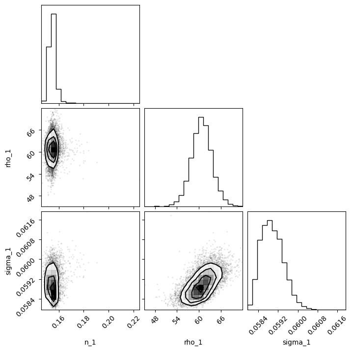
MCMC corner plot for power spectrum params (MCMC initialized at SVI median solution and
dense_mass=False):
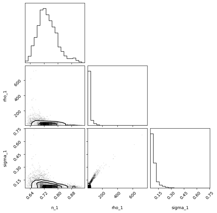
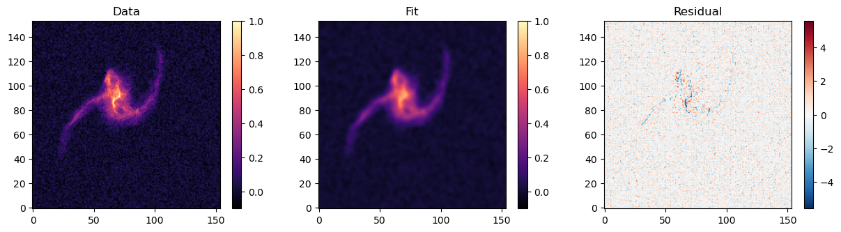
Both produce similar fits when compared to the data.
SVI final fit:

MCMC final fit:
Still not sure I am quite doing this right. Also, I would love a way to use NeuTraReparam on the combined guide to use it as a normalizing flow to get better/faster MCMC results. From what I can tell the guide would need to subclass off of AutoContinuous to allow for that. I just have no idea how to re-write the combined guide as this kind of class.
Your code is lgtm overall. I think you need to reparameterize the lat_a, lat_b sites to avoid such hierarchical dependency on a_loc, b_loc. e.g.
lat_a = a_loc + sample("lat_a_base", dist.Normal(loc=np.ones((nobs,)), scale=0.1))
1 Like
@CKrawczyk I think it’s enough to use the guide
def guide(data, shape, exposure_time):
    dep = dep_guide()
    ind = indep_guide(dep['n'], dep['sigma'], dep['rho'], shape)
Including obs into the guide will add an additional factor, which will cancel out the obs factor in the model. I.e. ELBO = E(p(y,z)-q(z)) rather than E(p(y,z)-q(y,z)).
In addition, like the comment above, it’s better to reparam your model:
pixels_real = scale * numpyro.sample('pixels_real_base', dist.Normal(0, 1))
1 Like