If I understand correctly, most inference algorithms used by NumPyro, such as Hamiltonian Monte Carlo, only require (log) densities up to a constant (ignoring the normalizing constant),
I was wondering why NumPyro distributions only provided a log_prob method, which implies computing the normalized distribution, and not also an unnormalized log-density method which doesn’t have the overhead of computing the normalization constant?
Using the unnormalized density could speed up computations by avoiding computing any normalization constants.
Is there any reason why using unnormalized densities would not work in NumPyro? Or are they already in use and have I missed something?
Hi @peter, in principle you’re right, that the density of a model needs only be normalized up to a constant, and that a some computations could in principle be sped up if the Distribution interface provided a .nonnormalized_log_prob() method that defaults to return self.log_prob(...). Here are some arguments in favor of exposing only .log_prob() (for sake of discussion ):
It’s helpful to have a model log density with interpretable units, so e.g. you can perform inference with two different distributions and compare marginal log likelihood of data. This is especially important in mixture models, where densities across mixture components need to agree. While you could toggle between normalized and non-normalized, the code gets tricky and opens up possibilities for bugs.
Savings are actually pretty rare. The reason is that the constant factor needs to be the same constant for all parameter values. I’ve seen a few practitioners misapply your intuition and create a CheapNormal distribution with log density (-0.5) * ((value - loc) / scale) ** 2 but forget that the normalizing constant depends on scale and their inference ends up garbage. This is the case in many distributions: the normalizing constant is actually not constant wrt all parameters, and you’d only save e.g. a multiplication by sqrt(2 * pi) or something here and there. I’d even wager that the savings are so rare and the cost in bugs so high, that offering the wider optimized interface would have net negative impact across the user base. But that’s just my intuition
In numpyro, I think that it is unlikely to get some performance improvement. When a jax program compiled with xla, those constant terms will become actual constants (thanks to xla optimization). There might be cases that such optimization does not trigger but it is rare I guess.
The reason why I was thinking that the non-normalized densities might speed up things is that Stan provides both normalized and non-normalized density functions for performance reasons: 20 Proportionality Constants | Stan User’s Guide
Also, I agree that dropping the constant on the Normal might only have minimal effect. I was thinking more along the lines of avoiding the normalization term in the Poisson distribution, which is slightly more complex and where the gammaln(value + 1) could be dropped (Please correct me if I’m wrong).
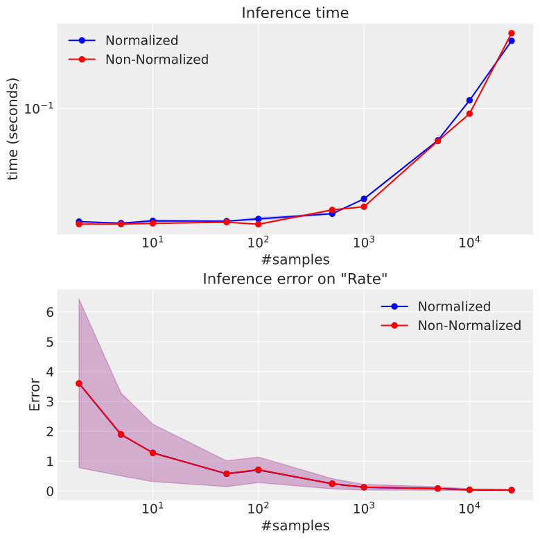
Since the proof of the pudding is in the eating, I decided to test compare the inference time of a non-normalized Poisson distribution vs the default NumPyro implementation, and indeed there is no significant difference:
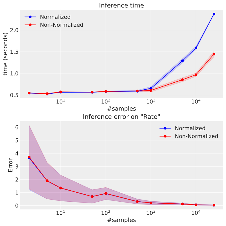
I decided to run some more experiments, and what is interesting is that when I turn on the progress bar with progress_bar=True, there seems to be a growing difference from 10^3 samples:
How could the progress bar have any effect on the differences in run-times? (When without progress bar I don’t notice any differences). At first I thought it was a fluke, but the result seem to be consistent with multiple runs/different seeds.
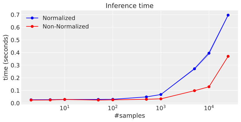
Another interesting observation: Using a HalfCauchy prior for the rate (instead of a Normal for the log_rate) Also shows a difference in inference time in favor for the non-normalized distribution:
I’ve observed a similar difference using dist.ImproperUniform(dist.constraints.positive, (), ())) as the rate distribution. The same here: I cannot explain this difference.
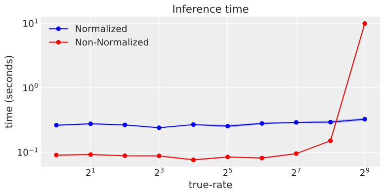
It seems however that the Non-Normalized Poisson likelihood is less stable for large rate values, and inference time becomes slow (x-axis is the ground-truth rate of the Poisson distribution to be fitted):
Interesting. When progress_bar=True, you can run mcmc._compile(...) first to compile the execution. Then you can measure the time for mcmc.run(...). Nevertheless, it seems to me that the difference is small. Thanks for the experiments - now I see that XLA is not as smart as I thought.
 ):
):