Hi all, I am trying to write a simple Linear Dynamical Model following Bishops definition (Chapter 13.3). In order to understand how to LDM works I first wanted to generate some toy data that I would know the parameters of and then try to predict them.
N_points = 500
A = 0.2
G = 0.5
C = 0.9
S = 1
mu0 = 0
V0 = 1

rng_key_toy_data = random.PRNGKey(33)
rng_key_toy_data, _ = random.split(rng_key_toy_data)

z1 = mu0 + random.normal(rng_key_toy_data) * V0

xs = []

z_prev = z1

for i in range(N_points):
    rng_key_toy_data, _ = random.split(rng_key_toy_data)
    z_t = random.normal(rng_key_toy_data) * G + z_prev * A

    rng_key_toy_data, _ = random.split(rng_key_toy_data)
    x_t = random.normal(rng_key_toy_data) * S + z_t * C
    z_prev = z_t
    xs += [x_t]
xs = jnp.array(xs)
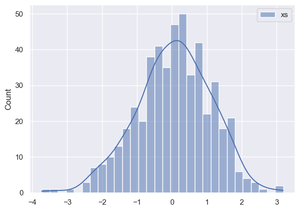
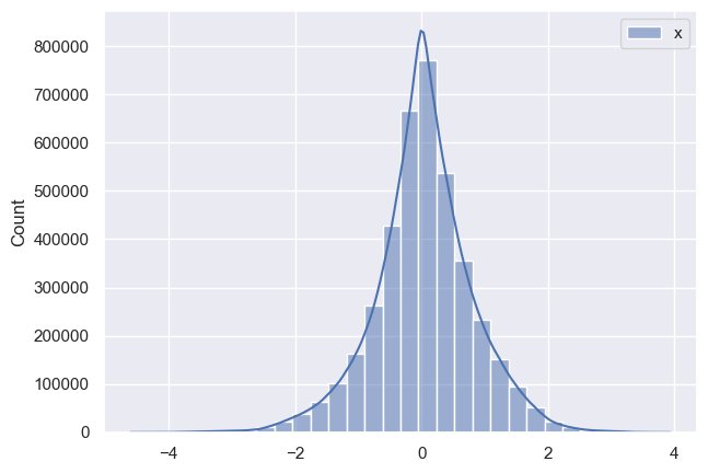
So here I have toy data that looks like this:
So far so good. Now I proceed to creating a model:
def modelToy(obs_data = None):
    L = obs_data.shape[0]

    # priors for parameteres
    A = numpyro.sample("A", dist.Normal(1, 1))
    C = numpyro.sample("C", dist.Normal(1, 1))

    G = numpyro.sample("G", FoldedStudentT(4, 0.1))
    S = numpyro.sample("S", FoldedStudentT(4, 0.1))

    V0 = numpyro.sample("V0", FoldedStudentT(4, 0.1))
    mu0 = numpyro.sample("mu0", dist.Normal(0, 1))
    sigma = numpyro.sample("sigma", FoldedStudentT(4, np.std(obs_data)))

    #initial z value
    z1 = numpyro.sample('z1', dist.Normal(mu0, V0))

    def chain(z_prev, _):
        z_t = numpyro.sample('z', dist.Normal(A*z_prev, G))
        x_t = numpyro.sample('xt', dist.Normal(C*z_t, S))
        return z_t, x_t

    _, x = scan(chain, z1, jnp.arange(L), length=L)
    numpyro.deterministic('x', x)

    numpyro.sample("obs", dist.Normal(x, sigma), obs=obs_data)
Here I was trying to follow hmm example. Now I run it:
rng_key = random.PRNGKey(0)
rng_key, rng_key_ = random.split(rng_key)

mcmc = MCMC(NUTS(model=modelToy, adapt_step_size=True, step_size=1e-2),
            num_samples=2000,
            num_warmup=10000,
            num_chains=4)
Now I want to see how posteriors look like and this is where I notice discrepancy:
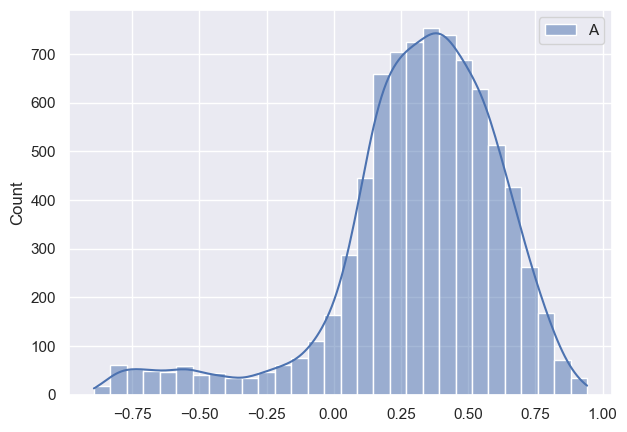
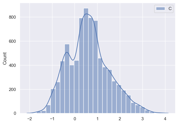
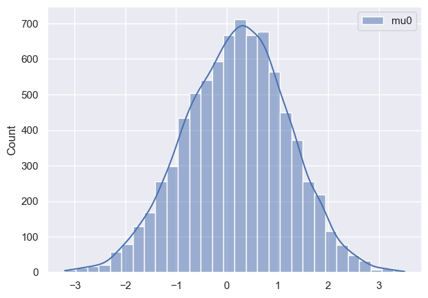
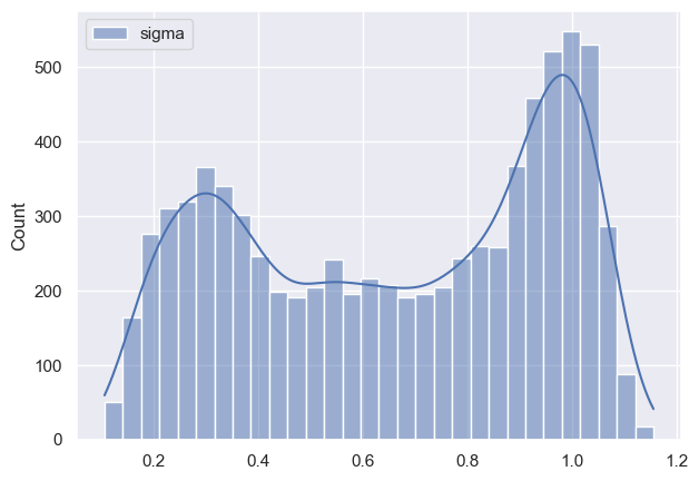
As it can be seen all parameters have very huge variance and appear bimodal (which I am not sure where it’s coming from, taking into account that I have modeled data). Initially I thought that maybe warm-up phase is not long enough, so I tried increasing it, but nothing changed much. Any suggestions what am I doing wrong?