So I have a relatively simple model - including a Dirichlet distribution - that works fine with MLE and MAP estimation (AutoDelta guide) but fails to do anything useful with any other guide. I tried AutoNormal, AutoDiagNormal, and a manually specified guide. All yielded similar (wrong) results. Unfortunately, I need uncertainty quantification, so simply doing MAP estimation / AutoDelta is not an option.
Not fully reproducible (can add that if it helps), but the gist of what I am doing:
def model_IR(x, y=None):
    arr = x.detach().cpu().numpy()
    assert np.all(arr[:-1] <= arr[1:]), "x input is assumed to be sorted"
    if y is not None:
        assert x.shape == y.shape

    steps = pyro.sample("steps", dist.Dirichlet(torch.ones_like(x)))  # flat prior over vector with positive entries that sums to one
    scale = pyro.sample("scale", dist.Beta(1, 1))  # flat prior over [0, 1] variable
    # probs is a (latent) monotonically increasing vector with probs[0] >= 0 and probs[-1] < 1.
    probs = torch.minimum(steps.cumsum(-1) * scale, torch.tensor(1 - 1e-7))  # I do not know why the clipping is necessary

    with pyro.plate("data", x.shape[0]):
        # observed binary outcomes, p(y=1) given by probs
        observation = pyro.sample("obs", dist.Bernoulli(probs=probs), obs=y)

def guide_IR(x, y=None):
    dirichlet_pars = pyro.param("dirichlet_pars", torch.ones_like(x), constraint=dist.constraints.positive)
    steps = pyro.sample("steps", dist.Dirichlet(dirichlet_pars))

    beta_alpha = pyro.param("beta_alpha", torch.tensor(1.0), constraint=dist.constraints.positive)
    beta_beta = pyro.param("beta_beta", torch.tensor(1.0), constraint=dist.constraints.positive)
    scale = pyro.sample("scale", dist.Beta(beta_alpha, beta_beta))

# SVI estimation, runs through but doesn't yield anywhere near correct results.
# I also tried guide_IR above and an AutoDiagNormal guide, all yielding similar (wrong) results.
# When I use AutoDelta(model_IR) here, I get the same (correct) result as with ML estimation.
guide = AutoNormal(model_IR)

scheduler = pyro.optim.MultiStepLR({'optimizer': torch.optim.Adam,
                         'optim_args': {'lr': 0.005},
                         'milestones': [20],
                         'gamma': 0.2})
svi = SVI(model=model_IR, guide=guide, optim=scheduler, loss=Trace_ELBO())
for i in range(5000):
    loss = svi.step(X_train, y_train, mle=mle)

predictive = Predictive(model_IR, guide=guide, num_samples=100)
svi_samples = predictive(X_train)
probs = svi_samples['scale'].squeeze().unsqueeze(-1) * svi_samples['steps'].squeeze().cumsum(-1)
Without going into the details, this is what a correct solution of variable “probs” on y axis plotted vs. x would look like in my test case (as correctly identified when doing MLE/MAP estimation): 0 in the left half, jumps to 1 in the right half (blue line; the black dashed line is just for reference).
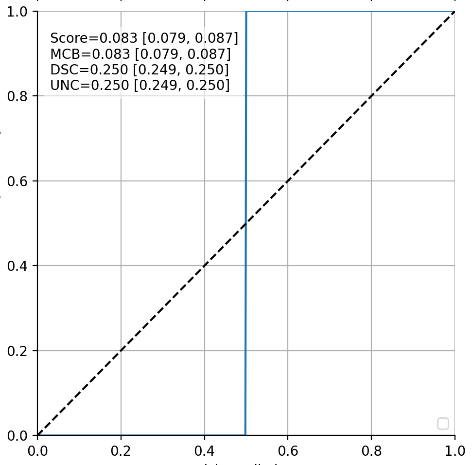
This is what’s estimated by SVI instead (in this case, using the AutoNormal guide): close to a diagonal.

Any ideas on how I might get closer to a correct solution are highly appreciated!
I believe I already do most if not all applicable things mentioned in the Tips and Tricks section of the SVI tutorial.
Am I correct in assuming that the model / prior cannot be the problem because it works with an AutoDelta guide?
Is it possible to evaluate the loss at the true solution and see whether I’m just seeing a local minimum and need to play around more with the optimization strategy? (Results were at least robust to different learning rates, LR scheduling yes/no, and different initialization attempts. So I am not overly optimistic about this.)
One thing that thoroughly confuses me is that when I perform inference using MCMC (NUTS, 4 chains, 1000 warmup steps + 1000 samples) I also receive results like in the second figure above. But MCMC is fully independent of the guide… so maybe the problem is not with the guide, after all? But how can the model/prior be at fault if it works nicely with the AutoDelta guide / MAP? Maybe the problem is somehow with how I use predictive in the end…? I am basically just interested in the distribution of the latent “probs” variable.