Stochastic Block Model using Pyro

Hi guys!

Might be a longer post, but I want to be specific :slight_smile:

I’m currently doing a research internship at the Technical University Munich (TUM) and working on Stochastic Block Models (SBMs). Since I am new to the topic of inference, I followed an example SBM implementation in the probabilistic framework edward1 (see here). This succeeded and was a nice way to start getting familiar with probabilistic modeling itself. However, Pyro seems to be more flexible and generally more user friendly for our purposes as to why we want to implement the SBM using Pyro.

However, I ran into some issues regarding parameter concentration values, dimensions, etc. and am having a difficult time debugging. In principle, I used the Pyro documentation to get familiar with models and guides and in particular this example on SVI.

I basically tried porting my SBM implementation of the famous karate club data set from edward to Pyro. To make things/info more accessible to you, have a look at my code from my GitHub directory (using Python 3.7 as base interpreter):

→ My probabilistic SBM approach (formulas) can be found here
→ My initial SBM implementation using edward can be found here
→ My attempt at a Pyro version can be found here.
Note, I have defined two guides guide_1 and guide_2. The first one matches more or less what I have found in the examples, the second one resembles more the solution based on edward.

As far as I have understood:

  • The model defines the general probabilistic structure and assumed random variable distribution
  • The guide defines the variational parameters, initializes them and prepares them for inference
  • SVI is then chosen as the inference algorithm

My questions:

  1. Have I correctly defined the model and guide?
  2. Have I correctly addressed the observed data and connected it to the model adjacency matrix? Is this the way how to do it?
  3. I tried debugging the code, however I run into value and dimension issues. Anyone see a fix?
  4. Optional: Can the SBM be defined more easily using a pyro.plate structure?

I am very curious and seem to understand more every day. I would greatly appreciate any help!

Thank you :slight_smile:

1 Like

Whoa, I am especially interested in SBM and graphon/graphing in general and also would like to learn and apply my knowledge to this field. @aladinD I am happy to take a look this weekend if this thread is still alive until then.

If anyone else has inputs for this, please jump in. This should be a cool topic to discuss. :slight_smile:

Edit: this reference is also relevant

2 Likes

Yes, this would be great!

There is a greater use case for SBMs and it would be optimal to solve most of the problem sets using Pyro :wink:

@aladinD Just looking at your implementation, here are some suggestions

Have I correctly defined the model and guide?

For the model, there are a few things missing:

  • You need to declare the event/batch dimensions of your priors. You can read tensor shapes tutorial for more information. If you unsure what to do, just simply call .to_event() for each prior. For example
Eta = pyro.sample("Eta", dist.Beta(0, 1).expand([K, K]).to_event())
  • It seems that you missed declaring shape (N,) for Z. You can use dist.Multinomial(...).expand([N]).to_event() if not sure what to do.

For the guides:

  • In the model, Eta has the shape K, K while in guide1 Eta has the shape K.
  • In the model, pi has the shape K while in guide1 pi has the shape K, K.
  • The categorical distribution in the guide1 has different support w.r.t. to the Multinomial distribution in the model.
  • All priors in model2 are not distributions. I guess you wanted to use dist.Delta(torch.nn.Sigmoid(eta_sigmoid_q)) at those places?
  • In model2, the support of Z is a vector of integers, while the output of softmax is a simplex. I am not sure what you wanted to do here. In the case of K=2, I guess you want to round the outputs of softmax to integers? (e.g. (0.3, 0.7) -> (0, 1)?)

Have I correctly addressed the observed data and connected it to the model adjacency matrix? Is this the way how to do it?

The svi.step(data) function needs to have the same signature as the definition of model/guide. So you need to provide data, nodes, K there (though I am not sure what nodes do in your model). In addition,

SVI(model=SBM_Model(data, nodes, K),
    guide=SBM_Guide_1(data, nodes, K),...)

should be

SVI(model=SBM_Model, guide=SBM_Guide_1,...)

I tried debugging the code, however I run into value and dimension issues. Anyone see a fix?

There are many things that are misspecified in your implementation, as pointed out above. I suggest working with the SVI tutorials again will be very helpful for you to understand how to do SVI inference in Pyro.

Can the SBM be defined more easily using a pyro.plate structure?

If you want to use it, you can do something like

with plate("N", N):
    Z = pyro.sample("Z", dist.Multinomial(total_count=1, probs=pi))

but it seems to me that plate is not needed for your model. Using .to_event() is enough in my opinion.

@fehiepsi Thank you very much for your reply and sorry for this rather late feedback!

I have clearly misunderstood some of Pyro’s fundamentals (model and notation wise) and am now working on an updated version of my SBM. I will post it shortly, so we can review it together! :smiley:

1 Like

@fehiepsi @fritzo

Hey there! :slight_smile:
This is our implementation so far, we took the Gaussian Mixture Model example as inspiration and have resolved the shape problems we initially had. Inference - or at least the SVI loop - seems to go through, however I do not see that the model has “learned” any parameters so far. The result seems to be a rather random membership vector Z which is also shown in the adjusted rand score we calculate in the end.

The main questions we have are basically

  1. Have we inferred correctly? (Using infer descrete, etc.)
  2. Do we successfully sample the “learned” parameters in the end.

Note that we saved our values in lists called “output” for debugging purposes. Maybe this is also useful for you. Here is our code:

# Pyro Environment Settings
pyro.enable_validation(True)
pyro.set_rng_seed(1)
pyro.clear_param_store()

def model(data, K):
    N = data.shape[0]

    # Eta
    with pyro.plate("eta_plate_1", K):
        with pyro.plate("eta_plate_2", K):
            eta_dist = dist.Beta(torch.ones([K, K]), torch.ones([K, K]))
            eta = pyro.sample("eta", eta_dist)

    # Membership Prior Pi
    pi_dist = dist.Dirichlet(concentration=torch.ones([K]))
    pi = pyro.sample("pi", pi_dist)

    # Community Association Z
    with pyro.plate("z_plate", N):
        z_dist = dist.Categorical(pi)
        z = pyro.sample("z", z_dist, infer={"enumerate": "parallel"})

    # Adjacency Matrix A
    with pyro.plate("a_plate_1", N):
        with pyro.plate("a_plate_2", N):
            a_dist = dist.Bernoulli(Vindex(Vindex(eta)[z, :])[:, z])
            a = pyro.sample("a", a_dist, obs=data)

def guide(data, K):
    N = data.shape[0]

    # Eta
    eta_1 = pyro.param("eta_1", torch.abs(torch.rand([K, K])), constraint=constraints.positive)
    eta_2 = pyro.param("eta_2", torch.abs(torch.randn([K, K])), constraint=constraints.positive)

    with pyro.plate("eta_plate_1", K):
        with pyro.plate("eta_plate_2", K):
            q_eta_dist = dist.Beta(eta_1, eta_2)
            q_eta = pyro.sample("eta", q_eta_dist)

    # Membership Prior Pi
    pi_conc = pyro.param("pi_conc", torch.abs(torch.rand(K)), constraint=constraints.positive)
    q_pi_dist = dist.Dirichlet(pi_conc)
    q_pi = pyro.sample("pi", q_pi_dist)

    # Community Association Z
    with pyro.plate("z_plate", N):
        q_z_dist = dist.Categorical(q_pi)
        q_z = pyro.sample("z", q_z_dist)

    # Adjacency Matrix A
    with pyro.plate("a_plate_1", N):
        with pyro.plate("a_plate_2", N):
            q_a_dist = dist.Bernoulli(Vindex(Vindex(q_eta)[q_z, :])[:, q_z])
            q_a = pyro.sample("a", q_a_dist)

# Data Set
testSet = 1

if testSet == 1:
    A_observed, Z_true = karate("~~data")
    A_observed = A_observed.astype(np.float32)
else:
    A_observed  = np.array([
        [0, 1, 1, 1, 1, 0, 0, 0, 0, 0],
        [1, 0, 1, 1, 1, 0, 0, 0, 0, 0],
        [1, 1, 0, 1, 1, 0, 0, 0, 0, 0],
        [1, 1, 1, 0, 1, 0, 0, 0, 0, 0],
        [1, 1, 1, 1, 0, 1, 0, 0, 0, 0],
        [0, 0, 0, 0, 1, 0, 1, 1, 1, 1],
        [0, 0, 0, 0, 0, 1, 0, 1, 1, 1],
        [0, 0, 0, 0, 0, 1, 1, 0, 1, 1],
        [0, 0, 0, 0, 0, 1, 1, 1, 0, 1],
        [0, 0, 0, 0, 0, 1, 1, 1, 1, 0],
    ], dtype=np.float32)

    Z_true = torch.tensor([1., 0., 1., 0., 1., 0., 1., 0., 1., 0.])

# Optimizer
adam_params = {"lr": 0.0005, "betas": (0.95, 0.999)}
adam_optimizer = Adam(adam_params)

# Tracing
trace = poutine.trace(model).get_trace(torch.tensor(A_observed), 2)
trace.compute_log_prob()
print(trace.format_shapes())

# Inference
svi = SVI(model,
          guide,
          adam_optimizer,
          loss=TraceEnum_ELBO(max_plate_nesting=2)
          )

# Learning
n_steps = 500

# Saving Values for Debugging`
output1=[]
output2=[]
output3=[]
output4=[]
output5=[]

for step in range(n_steps):
    print("Loss: ", svi.step(data=torch.tensor(A_observed), K=2))

    pi_curr = pyro.param("pi_conc")
    eta_1_curr = pyro.param("eta_1")
    eta_2_curr = pyro.param("eta_2")
    eta_curr = pyro.sample("eta_curr", dist.Beta(eta_1_curr, eta_2_curr))
    N = A_observed.shape[0]
    z_curr = pyro.sample("z_curr", dist.Categorical(probs=pi_curr), sample_shape=([N]))

    output1.append(pi_curr)
    output2.append(eta_curr)
    output3.append(z_curr)
    output4.append(eta_1_curr)
    output5.append(eta_2_curr)

guide_trace = poutine.trace(guide).get_trace(torch.tensor(A_observed), 2)  # record the globals
trained_model = poutine.replay(model, trace=guide_trace)  # replay the globals

def classifier(data, temperature=0):
    inferred_model = infer_discrete(trained_model, temperature=temperature,
                                    first_available_dim=-1)  # avoid conflict with data plate
    trace = poutine.trace(inferred_model).get_trace(data, 2)
    return trace.nodes["z"]["value"]

print("Classifier: ", classifier(torch.tensor(A_observed)))

# Information Extraction
for name, value in pyro.get_param_store().items():
    print(name, pyro.param(name))

print("Output 2 (Eta)", output2[-1])

pi_conc = pyro.param("pi_conc")
pi_calc = pyro.sample("pi_calc", dist.Dirichlet(concentration=pi_conc))
z_calc = pyro.sample("z_calc", dist.Categorical(probs=pi_calc), sample_shape=([N]))
print("z_calc", z_calc) # Looks good

print("ARS", adjusted_rand_score(z_calc, Z_true))

# Visualization
Z_pred = z_calc

G = nx.from_numpy_matrix(A_observed)
nx.draw(G, pos=nx.spring_layout(G), node_color=["red" if x==1 else "blue" for x in Z_pred])
plt.show()
nx.draw(G, pos=nx.spring_layout(G), node_color=["red" if x==1 else "blue" for x in Z_true])
plt.show()

Any help is greatly appreciated :slight_smile:

@aladinD Could you reformat the code. Currently, it does not indent as expected.

1 Like

Done!
Thanks for pointing out :slight_smile:

1 Like

Per our discussion:

  • we can’t use enumeration for this model
  • probably TraceGraph_ELBO will work
def guide(data, K):
    N = data.shape[0]
    eta_map = pyro.param("eta_map", torch.full((K, K), 0.5),
                         constraint=constraints.unit_interval)
    with pyro.plate("eta_plate_1", K):
        with pyro.plate("eta_plate_2", K):
            q_eta = pyro.sample("eta_map", dist.Delta(eta))
    pi_map = pyro.param("pi_map", torch.ones(K)/ K,
                        constraint=constraints.simplex)
    q_pi = pyro.sample("pi", dist.Delta(pi_map))
    ...

Hi,
I m also interested in the SBM implementation but unfortunately I struggle to fully comprehend Pyro’s complexity .
If I understand correctly you’re proposing a MAP guide instead of the full posteriors?
Is it the same as performing an AutoDelta guide?
Why isn’t enumeration possible and how do I instead infer the latent states of the categorical distribution?
cheers

Hi @cosmicc ,

we have solved our implementation issues and I will post a summary + example code for the Karate Club data set shortly! :slight_smile:

Thank you for reminding me!

2 Likes

Hello everyone! :smiley:

As promised, i give an update and summary on our findings regarding the SBM implementation in Pyro.

In general, we haven’t been able to obtain a fully-functioning SBM model using solely the tools and methods provided by Pyro itself. There are many reasons as to why and these themselves are quite dependent on the respective approach we tried using. Note that we decided for an SVI inference solution.

In our first model implementations as for instance, we focused on the GMM example as it is very similar to the SBM in its nature. However, here we encountered issues with the “learning” process. To make it short, membership inference worked well - at least for a very simple toy example with two communities - if and only if the Stochastic Block Matrix was initialized/learned properly in the first place. This resulted in us trying various approaches to accurately estimate the block matrix parameters using Pyro. In the end though, this has not worked at all meaning that we weren’t able to obtain a “closed-form” inference solution. We also tried using an auto_guide as suggested in the GMM documentation with the hope for a better parameter initialization, unfortunately without much success. The problem simply persisted in a more or less biased block matrix initialization we couldn’t get rid off.

Some other things we also considered were:

  • Switch to TraceGraph_ELBO to eliminate high variance we encountered during inference
  • Apply separate model/guide pairs for block matrix parameter learning and membership inference
  • Increase the number of particles (num_particles) in the loss settings for a more granular inference (note that this takes significantly more time in computing the solution)
  • MAP inference approach motivated by edward1 (TensorFlowProbability)
  • Variations in Multinomial/Categorical realizations of the model
  • Enumeration in very early models (mostly did not work because of dimensionality issues)

To summarize, inference results were quite frustrating. Either, we did not infer correctly or we ended up with a perfectly random solution, that is a membership probability of ~50% for either group. Also note that for debugging and testing reasons, we switched from the already simple karate club data set to an even simpler toy data set where two groups are connected to each other by only a single edge and the respective nodes in themselves are fully connected with each other. With that in mind, we were even more frustrated with the results as we could not have fabricated a more basic example as this one. Also, computation/inference time was exhaustingly long with some of above variations - such as the block matrix parameter learning + subsequent inference with increased num_particles - we tried.

Before giving the solution that now finally works, I first want to answer your questions @cosmicc.

If I understand correctly you’re proposing a MAP guide instead of the full posteriors? Is it the same as performing an AutoDelta guide?

A short answer to your question: Yes, AutoDelta should in principle equal a more or less “automated” MAP inference approach.

A more detailed answer: In above @fehiepsi 's post from Feb 2, he has given a “manual” MAP inference. What AutoDelta basically tries to achieve is a point estimate which is exactly what MAP inference basically is and what @fehiepsi has implemented. The reason why we additionally tried inference using the AutoDelta guide is because we combined it with an initialization process as described in the GMM example.

Unfortunately though, both methods did not yield satisfying inference results.

Why isn’t enumeration possible and how do I instead infer the latent states of the categorical distribution?

This is a very good question! In general, enumeration seems to be the most natural way to go for discrete latent variables in this case. However, we came across two major problems:

First, enumeration only supports a limited dimensionality, that is if you want to enumerate more than 25 variables, you have to apply some tricks. You can check the documentation for this provided here. As we wish to apply the SBM model for a larger-scale use case, this seems to be a more or less significant constraint w.r.t. plates parallelization, etc. where we are not sure how this would affect computation times and other things for our intended use-case.

Second, when using enumeration, indexing works a bit different. And this is exactly where we encountered most of the problems that subsequently affected other things in our code. In the definition of our adjacency matrix in the model, we are basically forced to use Vindex (don’t worry, this is also explained in above documentation link). To make it short, this led to some various problems regarding inference using our specified guide.

Current Solution
When we started looking for a probabilistic framework in order to implement the SBM, we wished for a very simple, easy to understand solution that relied on already existing widely used frameworks such as TensorFlow and PyTorch. Initially, Pyro seemed to provide all that and above all a very detailed documentation with many examples. However, for above stated reasons, the implementation of a simple Stochastic Block Model just would not work. I would not say that it is not possible as there are surely some variants and functionalities that are not explicitly detailed in the documentation, however after reviewing with @fehiepsi we now obtained an MCMC solution using a DiscreteHMCGibbs kernel. Please note that this exact implementation solution is not part of Pyro but of NumPyro. It works well, is very fast and most importantly correctly identifies memberships without any “good guess initializations”. Also note that NumPyro builds up on Google JAX which you have at least heard of recently if you are somewhat up to date with ML frameworks. As such, I would suggest to catch up on MCMC and HMC concepts in Pyro and then move on to NumPyro for the SBM realization.

Working SBM Example:

import jax
import jax.numpy as jnp
import numpyro
import numpyro.distributions as dist
from numpyro.infer import DiscreteHMCGibbs, MCMC, NUTS
import networkx as nx   # Version 1.9.1
from observations import karate
import matplotlib.pyplot as plt

def model(A, K):
    # Network Nodes
    n = A.shape[0]

    # Block Matrix Eta
    with numpyro.plate("eta1", K):
        with numpyro.plate("eta2", K):
            eta = numpyro.sample("eta", dist.Beta(1., 1.))

     # Group Memberships (Using a Multinomial Model)
     membership_probs = numpyro.sample("z_probs", dist.Dirichlet(concentration=jnp.ones(K)))
     with numpyro.plate("membership", n):
         sampled_memberships = numpyro.sample("sampled_z", dist.Categorical(probs=membership_probs))
         sampled_memberships = jax.nn.one_hot(sampled_memberships, K)

      # Adjacency Matrix
      p = jnp.matmul(jnp.matmul(sampled_memberships, eta), sampled_memberships.T)
      with numpyro.plate("rows", n):
          with numpyro.plate("cols", n):
               A_hat = numpyro.sample("A_hat", dist.Bernoulli(p), obs=A)

# Simple Toy Data
A = jnp.array([
    [0, 1, 1, 1, 1, 0, 0, 0, 0, 0],
    [1, 0, 1, 1, 1, 0, 0, 0, 0, 0],
    [1, 1, 0, 1, 1, 0, 0, 0, 0, 0],
    [1, 1, 1, 0, 1, 0, 0, 0, 0, 0],
    [1, 1, 1, 1, 0, 1, 0, 0, 0, 0],
    [0, 0, 0, 0, 1, 0, 1, 1, 1, 1],
    [0, 0, 0, 0, 0, 1, 0, 1, 1, 1],
    [0, 0, 0, 0, 0, 1, 1, 0, 1, 1],
    [0, 0, 0, 0, 0, 1, 1, 1, 0, 1],
    [0, 0, 0, 0, 0, 1, 1, 1, 1, 0]])
Z = jnp.array([0, 0, 0, 0, 0, 1, 1, 1, 1, 1])
K = 2

# Inference
kernel = DiscreteHMCGibbs(NUTS(model))
mcmc = MCMC(kernel, num_warmup=1500, num_samples=2500)
mcmc.run(jax.random.PRNGKey(0), A, K)
mcmc.print_summary()
Z_infer = mcmc.get_samples()["sampled_z"]
Z_infer = Z_infer[-1]
print("Inference Result", Z_infer)
print("Original Memberships", Z)

# Visualization
G = nx.from_numpy_matrix(A)
plt.figure(figsize=(10,4))
plt.subplot(121)
nx.draw(G, pos=nx.spring_layout(G), node_color=["red" if x==1 else "blue" for x in Z])
plt.title("Original Network")

plt.subplot(122)
nx.draw(G, pos=nx.spring_layout(G), node_color=["red" if x==1 else "blue" for x in Z_infer])
plt.title("Inferred Network")
plt.show()

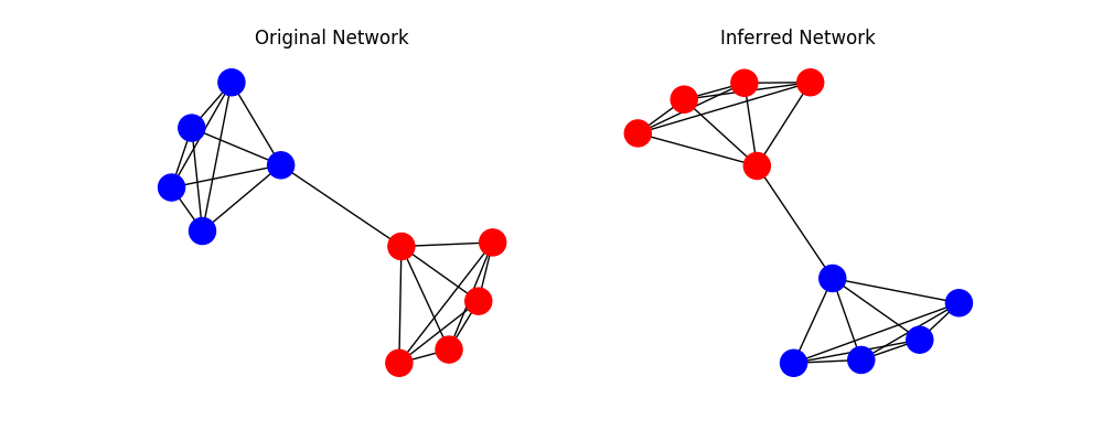
We obtain the following result:

sample: 100%|██████████| 2000/2000 [00:15<00:00, 131.59it/s, 7 steps of size 5.16e-01. acc. prob=0.89]

                  mean       std    median      5.0%     95.0%     n_eff     r_hat
    eta[0,0]      0.78      0.07      0.79      0.65      0.89   1524.15      1.00
    eta[0,1]      0.07      0.05      0.06      0.00      0.14   1365.40      1.00
    eta[1,0]      0.07      0.05      0.06      0.00      0.15   1937.00      1.00
    eta[1,1]      0.78      0.08      0.79      0.66      0.90   1841.28      1.00
sampled_z[0]      0.00      0.00      0.00      0.00      0.00       nan       nan
sampled_z[1]      0.00      0.00      0.00      0.00      0.00       nan       nan
sampled_z[2]      0.00      0.00      0.00      0.00      0.00       nan       nan
sampled_z[3]      0.00      0.00      0.00      0.00      0.00       nan       nan
sampled_z[4]      0.00      0.00      0.00      0.00      0.00       nan       nan
sampled_z[5]      1.00      0.00      1.00      1.00      1.00       nan       nan
sampled_z[6]      1.00      0.00      1.00      1.00      1.00       nan       nan
sampled_z[7]      1.00      0.00      1.00      1.00      1.00       nan       nan
sampled_z[8]      1.00      0.00      1.00      1.00      1.00       nan       nan
sampled_z[9]      1.00      0.00      1.00      1.00      1.00       nan       nan
z_probs[0,0]      0.67      0.23      0.70      0.33      1.00   1785.41      1.00
z_probs[0,1]      0.33      0.23      0.30      0.00      0.67   1785.41      1.00
z_probs[1,0]      0.66      0.24      0.71      0.31      1.00   1393.45      1.00
z_probs[1,1]      0.34      0.24      0.29      0.00      0.69   1393.45      1.00
z_probs[2,0]      0.67      0.25      0.72      0.31      1.00   2086.85      1.00
z_probs[2,1]      0.33      0.25      0.28      0.00      0.69   2086.85      1.00
z_probs[3,0]      0.67      0.24      0.71      0.32      1.00   1866.58      1.00
z_probs[3,1]      0.33      0.24      0.29      0.00      0.68   1866.58      1.00
z_probs[4,0]      0.67      0.23      0.71      0.34      1.00   1572.49      1.00
z_probs[4,1]      0.33      0.23      0.29      0.00      0.66   1572.49      1.00
z_probs[5,0]      0.33      0.24      0.29      0.00      0.69   1532.02      1.00
z_probs[5,1]      0.67      0.24      0.71      0.31      1.00   1532.02      1.00
z_probs[6,0]      0.35      0.24      0.32      0.00      0.70   2433.68      1.00
z_probs[6,1]      0.65      0.24      0.68      0.30      1.00   2433.68      1.00
z_probs[7,0]      0.33      0.24      0.29      0.00      0.69   1966.93      1.00
z_probs[7,1]      0.67      0.24      0.71      0.31      1.00   1966.93      1.00
z_probs[8,0]      0.33      0.24      0.29      0.00      0.68   1725.91      1.00
z_probs[8,1]      0.67      0.24      0.71      0.32      1.00   1725.91      1.00
z_probs[9,0]      0.33      0.23      0.30      0.00      0.66   1216.91      1.00
z_probs[9,1]      0.67      0.23      0.70      0.34      1.00   1216.91      1.00

Inference Result [1 1 1 1 1 0 0 0 0 0]
Original Memberships [0 0 0 0 0 1 1 1 1 1]

Please Note:
SBM models - or at least in the current implementation provided here - are prone to two things: Label-Switching and Higher-Lower-Splits. As you can see, the labels are switched in this case which is not a problem at all. However, once you try to apply the solution to the Karate Club, you have to deal with higher and lower splittings, that is the model prefers nodes of higher degree over lower ones and thus constructs the groups as such. This is widely known and I suggest to read more on that on page 21 of this document.

I would like to thank @fehiepsi very much for his hugely appreciated help! We gained more insight into the Pyro mechanics and the solution we obtained together is pretty satisfying for our current use-case :smiley:

If there are any more questions, I am open to discuss them. For now, I hope the NumPyro solution works for you, too @cosmicc.

5 Likes

@aladinD Thank you for this very well written post. I never really bothered checking out Jax. Thus thanks for pointing me towards this impressive and promising looking tech (I hate the permanent transitions between pandas dataframes, xarrays, numpy arrays, pytorch tensors).
Will definitely have an in depth inspection of the overall algorithm and there will definitely be more questions rising up ;).

@aladinD FYI, this new algorithm seems to be pretty suitable for SBM. I would expect it will give a better result than DiscreteHMCGibbs. :slight_smile:

1 Like

Hi, the Model seems pretty solid. The Model can also be easily extended to a mixed membership model by using a second categorical distribution and exchanging one of the vectors with the corresponding 1-hot encoded vector in the matrix multiplication.
I am thinking about including a time dependency as part of the block mapping process in suitable and sensitive manner. Do you guys have any hints?

@fehiepsi shouldn’t we take the mode instead of the last sampled latent states (MAP)? Do you have any knowledge/publications on treating the block number as additional random variable and performing inference?

I’m not sure I understand. Which inference algorithm that you mentioned? For MCMC algorithms, what we got is a collection of latent samples, rather than a single value. If you are performing MAP inference, then the MAP point is the mode of the posterior.

treating the block number as additional random variable

I recalled that the Bayesian stochastic blockmodeling paper setups a Bayesian model for the number of blocks.

I meant this part of the code. Shouldn’t we take the mode of mcmc.getsamples()[‘sampled_z’] instead of the latest sampled point as a more robust and meaningful latent state estimation? or am I mistaken. I’m still relatively new to the whole probabilistic ML spectrum but find it extremely fascinating and powerful :). Thanks for the link.

It is constant during sampling process (you can look at the summary statistics in that comment), so taking the last value is fine IMO.

ah, I get your point. On my dataset the sampled traces where alternating between states, though in each trace there were always dominating states. The latest point was mostly working (matching the MAP) but I decided to switch to the mode to be sure.