Specifically in the section “Regression Model with Measurement Error”, where the measurement error is introduced to the model.
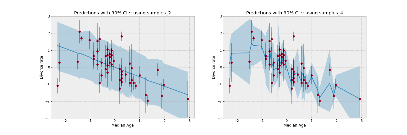
If we observe the figure of the residuals when the errors are introduced, there is a clear decrease in the difference between the predicted and the experimental value. However if we plot “Divorce rate” vs “Median Age” (see figure below), or vs “Marriage Rate” we see a somewhat strange behavior, there is really no linear regression. Is this expected behavior? or am I missing something, if possible I would like to be clarified.
The second question is, when you make the prediction using the “Predictive” function with the “model_se” model, the argument “divorce_sd=dset.DivorceScaledSD.values” is used, which is one of the results to be estimated together with “divorce”, and therefore cannot be used to predict. Is this OK?
divorce_rate = mu + sigma * numpyro.sample('divorce_rate', dist.Normal(0, 1).expand(mu.shape))
which is one of the results to be estimated
It seems to me that model_se only has divorce as an observed node. If you want to predict divorce_sd, then you need to add some generative code for divorce_sd
I’m starting in the Bayesian world and I do it directly with numpyro, so if I get lost with something theoretical or technical even if it’s obvious, please forgive me.
I guess the result will be more linear if we replace
The changes you suggest to make in the “model_se” do not change the behavior of “predictions_4”:
which is the evaluation used to make the predictions of “dset.DivorceScaled.values”. This non-linear behavior (which in my opinion is not correct), explains the drastic decrease of the residuals with respect to “model 3”.
The fact that this is a suspicious behavior can also be analyzed by comparing the regression coefficients [“a”, “bA”, “bM”] obtained with “model 3” and “model 4”. As it is emphasized in the text of the example and in the book, these coefficients do not differ much from each other, so I think that the prediction made with the same linear model (mu = a + bM * marriage + bA * age) in both cases cannot differ so much, as it is represented in the figure of the residuals.
divorce_sd = numpyro.sample(…, obs=divorce_sd)
From my basic knowledge it looks good to me, so the model would be generative (and predictive) for “divorce_rate” and “divorce_sd”.
Hi @Ubaldo, I think we are doing linear regression w.r.t. 2 variables, while the plot only shows linear relationship with 1 variable. Does it explain what you observed?
import numpy as np
import matplotlib.pyplot
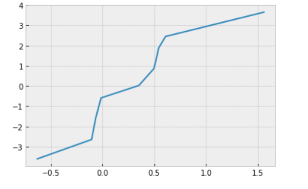
x = np.sort(np.random.randn(10))
y = np.sort(np.random.randn(10))
z = x + 2 * y
plt.plot(x, z)
plt.show()
Hi @fehiepsi,
You are totally right, I was working with another example (one-dimensional) parallel to this one and I ended up mixing things up, sorry for the confusion.
Please consider the following example [gist]. My doubt remains the same as in the first post, how to do the predictive analysis with the model and the “Predictive” function, or the alternative “Effect Handlers”. The example consists of a linear regression with a single independent variable, where errors in the measurement of “x” and “y” are considered.
Following the suggestion you made above I consider the error of “y” as an independent node, which allows me to make the predictions and that these are not dependent on that observable. You can see in the example that the coefficients of the linear regression are much better estimated with the model that considers the errors. My doubt comes, when I want to make predictions, making use of the function “Predictive”, the results differ from the linear behavior that is being estimated. There is something I am not considering correctly, and I cannot see what it is.
Hi @Ubaldo, it does not seem to me that model_xyerror is a linear model of y w.r.t. X. y heuristically is a noise version of sigma * y_true + beta_0 + beta_1 * X_true, where X_true is a noise version of X. Taking an example similar to the one in my last comment z = x + y where y = np.random.randn(10): because y is noise, you can think of z as a noise version of x. But it is clear from the plot that z does not have a linear relationship with x. Actually, X_true and y_true does not have a linear relationship w.r.t. X, so you can’t expect the noisy version y has a linear relationship w.r.t. X.
I think that by wanting to go one step forward I have been able to make mistakes, I will take a step back and build a model that only contemplates the error in the independent variable (covariate) and that I will call “model_xerror”. I’ll try to describe what I think I’m doing, so you can see if I’m making a theoretical error besides the one I might be making technically.
This problem is similar to when we have “missing values”, in our case we do not know “X_true”, but we know the values of the measurements (“X”) with the associated noise of the measurement: “X = X_true ± sigma_X”. Then we will try to estimate the distribution of “X_true” assuming that it is one more parameter of the model, to add flexibility to the model we will incorporate a hyperparameter associated to the experimental noise (“sigma_X”) and another to the mean. Assuming a linear relationship between the variables covariate and the outcome, that by construction we know that it is fulfilled, our model would be something like this:
### model ( model_xerror) ###

beta ~ Normal(0., 100.).shape([2]))
sigma ~ Exponential(1)

# true x
X_true_mu  ~ Normal(0., 100)
X_true_eta ~ HalfNormal(20)
X_true ~ Normal(X_true_mu, X_true_eta).shape([X.shape])
obs_X  ~ Normal(X_true, sigma_X) #likelihood of x , obs=x

# model
mu = beta[0] * X_true + beta[1]

obs ~ Normal(mu, sigma)  #likelihood of y, obs=y
In this way I can determine the “theoretical” parameters with which we generate the regression, you can see it in the [gist]. But I still can’t make the predictions, using “Predictive”.
@Ubaldo If you worried about Predictive, you can take one posterior sample and compute the prediction step-by-step. Please let me know if you observe something wrong. If you worried about why y_pred does not have a linear relationship w.r.t. X, then as I mentioned above: X_true ~ P(X_true | X, y) (assume other parameters X_true_mu, X_true_eta are constant, otherwise the situation is even more complicated) does not have a linear relationship w.r.t. X.
If the model is
X_true ~ Normal(0, 1)
X ~ Normal(X_true, 1)
, then P(X_true | X) ~ Normal(aX + b, c) for some a, b, c. So the mean of X_true will have a linear relationship with X. However, when y is involved, I don’t see why X_true ~ P(X_true | X, y) will have a linear relationship with X.
I think there is no issue with your code and the result is expected (as far as I see). What do you think?