TL;DR - The ELBO of my Sigmoid Belief Network is decreasing, and the resulting parameters appear to learn inverted binomials, I don’t know why that’s happening but would like to fix it and improve correlation structure of generated samples.
Solution: The loss is the negative ELBO, thanks @jpchen, also it turned out I had forgotten a minus sign in the sigmoid function, causing my code to perform poorly.
Context
I am currently attempting to build a Sigmoid Belief Network (SBN; Neil, 1992). The full code is attached at the bottom of this post, note that it is derived from the Sparse Gamma Deep Exponential Family example. The network looks as follows:
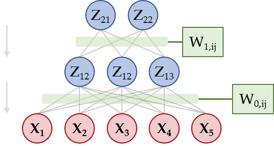
Here, the Z variables are latent binomials, and the X variables are observed binomials. The values of parents determine the p parameter for the next layer, through a set of weights. In order to have proper p values, that is in (0,1), we calculate p = sigmoid(Z'W).
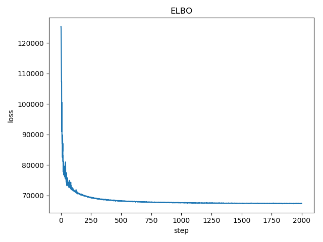
Now what I’m running into is that the value for my TraceGraph_ELBO loss is decreasing, rather than increasing – as it forms a lower bound on the likelihood we would like it as large as possible. See figure below.
For clarification; in order to compare the learned parameters, I sample a data set and compare the conditional and base probabilities between the true and sampled data.
The base probabilities appear to be inverted (that is, P(X=1) becomes P(X=0)) and most correlation structure is lost between the variables.
I’m looking to have the ELBO increase in the hopes that it will improve the performance of my model.
Best regards,
Scipio
Full code
import os
import sys
import argparse

import numpy as np
import torch
from pathlib import Path
from matplotlib import pyplot as plt
import pandas as pd

import torch.utils.data
import torch.optim as optim
import xlsxwriter

import pyro
from pyro import poutine
import pyro.optim as optim
from pyro.distributions import Bernoulli, Normal
from pyro.contrib.autoguide import AutoDiagonalNormal, AutoGuideList, AutoDiscreteParallel
from pyro.infer import SVI, TraceGraph_ELBO

torch.set_default_tensor_type('torch.FloatTensor')
pyro.enable_validation(True)
pyro.clear_param_store()
# pyro.util.set_rng_seed(26011994)

def sigmoid(x):
    return 1/(1+np.exp(x))


class SigmoidBeliefDEF(object):
    def __init__(self):
        # define the sizes of the layers in the deep exponential family
        self.top_width = 2
        self.bottom_width = 3
        self.data_size = 5
        # define hyperparameters that control the prior
        self.p_z = torch.tensor([0.7, 0.3])
        self.mu_w = torch.tensor(0.0)
        self.sigma_w = torch.tensor(3.0)
        # define parameters used to initialize variational parameters
        self.z_mean_init = 0.0
        self.z_sigma_init = 0.5
        self.w_mean_init = 0.0
        self.w_sigma_init = 2.0
        self.softplus = torch.nn.Softplus()

    # define the model
    def model(self, x):
        x_size = x.size(0)

        # sample the global weights
        with pyro.plate("w_top_plate", self.top_width * self.bottom_width):
            w_top = pyro.sample("w_top", Normal(self.mu_w, self.sigma_w))
        with pyro.plate("w_bottom_plate", self.bottom_width * self.data_size):
            w_bottom = pyro.sample("w_bottom", Normal(self.mu_w, self.sigma_w))


        # sample the local latent random variables
        # (the plate encodes the fact that the z's for different data points are conditionally independent)
        with pyro.plate("data", x_size):
            z_top = pyro.sample("z_top", Bernoulli(self.p_z).expand([self.top_width]).to_event(1))
            # note that we need to use matmul (batch matrix multiplication) as well as appropriate reshaping
            # to make sure our code is fully vectorized
            w_top = w_top.reshape(self.top_width, self.bottom_width) if w_top.dim() == 1 else \
                w_top.reshape(-1, self.top_width, self.bottom_width)
            mean_bottom = torch.sigmoid(torch.matmul(z_top, w_top))
            z_bottom = pyro.sample("z_bottom", Bernoulli(mean_bottom).to_event(1))

            w_bottom = w_bottom.reshape(self.bottom_width, self.data_size) if w_bottom.dim() == 1 else \
                w_bottom.reshape(-1, self.bottom_width, self.data_size)
            mean_obs = torch.sigmoid(torch.matmul(z_bottom, w_bottom))

            # observe the data using a Bernoulli likelihood
            pyro.sample('obs', Bernoulli(mean_obs).to_event(1), obs=x)

    # define our custom guide a.k.a. variational distribution.
    def guide(self, x):
        x_size = x.size(0)

        # helper for initializing variational parameters
        def rand_tensor(shape, mean, sigma):
            return mean * torch.ones(shape) + sigma * torch.randn(shape)

        # define a helper function to sample z's for a single layer
        def sample_zs(name, width):
            # Sample parameters
            p_z_q = pyro.param("p_z_q_%s" % name,
                               lambda: rand_tensor((x_size, width), self.z_mean_init, self.z_sigma_init))
            p_z_q = torch.sigmoid(p_z_q)
            # Sample Z's
            pyro.sample("z_%s" % name, Bernoulli(p_z_q).to_event(1))

        # define a helper function to sample w's for a single layer
        def sample_ws(name, width):
            # Sample parameters
            mean_w_q = pyro.param("mean_w_q_%s" % name,
                                  lambda: rand_tensor(width, self.w_mean_init, self.w_sigma_init))
            sigma_w_q = pyro.param("sigma_w_q_%s" % name,
                                   lambda: rand_tensor(width, self.w_mean_init, self.w_sigma_init))
            sigma_w_q = self.softplus(sigma_w_q)
            # Sample weights
            pyro.sample("w_%s" % name, Normal(mean_w_q, sigma_w_q))

        # sample the global weights
        with pyro.plate("w_top_plate", self.top_width * self.bottom_width):
            sample_ws("top", self.top_width * self.bottom_width)
        with pyro.plate("w_bottom_plate", self.bottom_width * self.data_size):
            sample_ws("bottom", self.bottom_width * self.data_size)

        # sample the local latent random variables
        with pyro.plate("data", x_size):
            sample_zs("top", self.top_width)
            sample_zs("bottom", self.bottom_width)


def main(args):
    dataset_path = Path(r"C:\Users\posc8001\Documents\DEF\Data\Simulation_1")
    file_to_open = dataset_path / "small_data.csv"
    f = open(file_to_open)
    data = torch.tensor(np.loadtxt(f, delimiter=',')).float()
    sigmoid_belief_def = SigmoidBeliefDEF()

    # Specify hyperparameters of optimization
    learning_rate = 0.5
    momentum = 0.05
    opt = optim.AdagradRMSProp({"eta": learning_rate, "t": momentum})

    # Specify parameters of sampling process
    n_samp = 100000

    # Specify the guide
    guide = sigmoid_belief_def.guide

    # Specify Stochastic Variational Inference
    svi = SVI(sigmoid_belief_def.model, guide, opt, loss=TraceGraph_ELBO())

    # we use svi_eval during evaluation; since we took care to write down our model in
    # a fully vectorized way, this computation can be done efficiently with large tensor ops
    svi_eval = SVI(sigmoid_belief_def.model, guide, opt,
                   loss=TraceGraph_ELBO(num_particles=args.eval_particles, vectorize_particles=True))

    # the training loop
    losses, final_w_bottom = [], []
    final_p_z_0 = []
    final_w_top = []
    final_sig_w_top = []
    sample = []
    final_sig_w_bottom = []

    for i in range(15):
        final_w_bottom.append([])

    for i in range(15):
        final_sig_w_bottom.append([])

    for i in range(2):
        final_p_z_0.append([])

    for i in range(6):
        final_w_top.append([])

    for i in range(6):
        final_sig_w_top.append([])

    for k in range(args.num_epochs):
        losses.append(svi.step(data))

        for i in range(2):
            final_p_z_0[i].append(torch.sigmoid(pyro.param("p_z_q_top")[:, i].mean()))

        for i in range(6):
            final_w_top[i].append(pyro.param("mean_w_q_top")[i].item())

        for i in range(15):
            final_w_bottom[i].append(pyro.param("mean_w_q_bottom")[i].item())

        if k % args.eval_frequency == 0 and k > 0 or k == args.num_epochs - 1:
            loss = svi_eval.evaluate_loss(data)
            print("[epoch %04d] training elbo: %.4g" % (k, loss))

        # if k == args.num_epochs - 1:
        #     # Sample fake data set
        #     p_z_top_1 = torch.sigmoid(pyro.param("p_z_q_top")[:, 0].mean())
        #     p_z_top_2 = torch.sigmoid(pyro.param("p_z_q_top")[:, 1].mean())
        #
        #     w1_z_bottom_1 = pyro.param("mean_w_q_top")[0].item()
        #     w1_z_bottom_2 = pyro.param("mean_w_q_top")[1].item()
        #     w1_z_bottom_3 = pyro.param("mean_w_q_top")[2].item()
        #     w2_z_bottom_1 = pyro.param("mean_w_q_top")[3].item()
        #     w2_z_bottom_2 = pyro.param("mean_w_q_top")[4].item()
        #     w2_z_bottom_3 = pyro.param("mean_w_q_top")[5].item()
        #
        #     w1_x_1 = pyro.param("mean_w_q_bottom")[0].item()
        #     w1_x_2 = pyro.param("mean_w_q_bottom")[1].item()
        #     w1_x_3 = pyro.param("mean_w_q_bottom")[2].item()
        #     w1_x_4 = pyro.param("mean_w_q_bottom")[3].item()
        #     w1_x_5 = pyro.param("mean_w_q_bottom")[4].item()
        #     w2_x_1 = pyro.param("mean_w_q_bottom")[5].item()
        #     w2_x_2 = pyro.param("mean_w_q_bottom")[6].item()
        #     w2_x_3 = pyro.param("mean_w_q_bottom")[7].item()
        #     w2_x_4 = pyro.param("mean_w_q_bottom")[8].item()
        #     w2_x_5 = pyro.param("mean_w_q_bottom")[9].item()
        #     w3_x_1 = pyro.param("mean_w_q_bottom")[10].item()
        #     w3_x_2 = pyro.param("mean_w_q_bottom")[11].item()
        #     w3_x_3 = pyro.param("mean_w_q_bottom")[12].item()
        #     w3_x_4 = pyro.param("mean_w_q_bottom")[13].item()
        #     w3_x_5 = pyro.param("mean_w_q_bottom")[14].item()
        #
        #     for samp in range(n_samp):
        #         ztop_1 = np.random.binomial(n=1, p=p_z_top_1.detach(), size=1)
        #         ztop_2 = np.random.binomial(n=1, p=p_z_top_2.detach(), size=1)
        #
        #         p_zbottom_1 = sigmoid(w1_z_bottom_1 * ztop_1 + w2_z_bottom_1 * ztop_2)
        #         p_zbottom_2 = sigmoid(w1_z_bottom_2 * ztop_1 + w2_z_bottom_2 * ztop_2)
        #         p_zbottom_3 = sigmoid(w1_z_bottom_3 * ztop_1 + w2_z_bottom_3 * ztop_2)
        #
        #         zbottom_1 = np.random.binomial(n=1, p=p_zbottom_1, size=1)
        #         zbottom_2 = np.random.binomial(n=1, p=p_zbottom_2, size=1)
        #         zbottom_3 = np.random.binomial(n=1, p=p_zbottom_3, size=1)
        #
        #         p_x_1 = sigmoid(w1_x_1 * zbottom_1 + w2_x_1 * zbottom_2 + w3_x_1 * zbottom_3)
        #         p_x_2 = sigmoid(w1_x_2 * zbottom_1 + w2_x_2 * zbottom_2 + w3_x_2 * zbottom_3)
        #         p_x_3 = sigmoid(w1_x_3 * zbottom_1 + w2_x_3 * zbottom_2 + w3_x_3 * zbottom_3)
        #         p_x_4 = sigmoid(w1_x_4 * zbottom_1 + w2_x_4 * zbottom_2 + w3_x_4 * zbottom_3)
        #         p_x_5 = sigmoid(w1_x_5 * zbottom_1 + w2_x_5 * zbottom_2 + w3_x_5 * zbottom_3)
        #
        #         x_1 = np.random.binomial(n=1, p=p_x_1, size=1)
        #         x_2 = np.random.binomial(n=1, p=p_x_2, size=1)
        #         x_3 = np.random.binomial(n=1, p=p_x_3, size=1)
        #         x_4 = np.random.binomial(n=1, p=p_x_4, size=1)
        #         x_5 = np.random.binomial(n=1, p=p_x_5, size=1)
        #
        #         sample.append([x_1, x_2, x_3, x_4, x_5])
        #
        #     workbook = xlsxwriter.Workbook('sampled_data.xlsx')
        #     worksheet = workbook.add_worksheet()
        #
        #     row = 0
        #     col = 0
        #
        #     for x1, x2, x3, x4, x5 in (sample):
        #         worksheet.write(row, col, x1)
        #         worksheet.write(row, col + 1, x2)
        #         worksheet.write(row, col + 2, x3)
        #         worksheet.write(row, col + 3, x4)
        #         worksheet.write(row, col + 4, x5)
        #         row += 1

    plt.plot(losses)
    plt.title("ELBO")
    plt.xlabel("step")
    plt.ylabel("loss");
    plt.show()

    for i in range(final_p_z_0.__len__()):
        plt.plot(final_p_z_0[i])
        plt.title("P Z_top_" + (i+1).__str__())
        plt.show()

    for i in range(final_w_top.__len__()):
        plt.plot(final_w_top[i])
        plt.title("Mean W_top_" + (i+1).__str__())
        plt.show()

    for i in range(final_w_bottom.__len__()):
        plt.plot(final_w_bottom[i])
        plt.title("Mean W_bottom_" + (i+1).__str__())
        plt.show()


if __name__ == '__main__':
    assert pyro.__version__.startswith('0.3.0')
    # parse command line arguments
    parser = argparse.ArgumentParser(description="parse args")
    parser.add_argument('-n', '--num-epochs', default=10000, type=int, help='number of training epochs')
    parser.add_argument('-ef', '--eval-frequency', default=25, type=int,
                        help='how often to evaluate elbo (number of epochs)')
    parser.add_argument('-ep', '--eval-particles', default=200, type=int,
                        help='number of samples/particles to use during evaluation')
    parser.add_argument('--auto-guide', action='store_true', help='whether to use an automatically constructed guide')
    args = parser.parse_args()
    model = main(args)