Simple BNN NUTS sampling

[JuanVacaciones]

Hello community,

I am new to Bayesian models and to pyro (and numpyro). I am trying to use a small Bayesian Network on simple synthetic data, with no success so far.

I am trying to reproduce this simple example with a simple BNN from this tutorial.
The model and training procedure is in the minimal example below.

The problem I am facing is the following:

• There is no noise in the data generated, so I would like to specify a small variance in the output, hence the small sigma scale in the last Normal prior. Is it the correct way to do it ?
• If I keep a scale with a Gamma prior as in the numpyro tutorial, my model is too simple with high variance and does not fit the data
• If I use a small prior on the scale, the NUTS has a large number of steps (3000/3000 [04:38<00:00, 10.76it/s, 1023 steps of size 1.62e-03. acc. prob=0.93) and the final model does not fit the data (see attached image)

Any idea of what is wrong in my model or training procedure?

Thanks.

import jax.numpy as jnp
import jax.random as random
from jax import vmap

import numpy as np
import numpyro
from numpyro import handlers
import numpyro.distributions as distnumpyro
from numpyro.infer import MCMC as MCMCnumpyro
from numpyro.infer import NUTS as NUTSnumpyro
from numpyro.infer import Predictive as PredictiveNumpyro
import os
from collections import namedtuple
import time
import plotly.graph_objects as go
from collections import namedtuple


def model_bnn_numpyro(X, Y, hid_dim=50, out_dim=1):
    N, D_X = X.shape
    D_H = hid_dim
    D_Y = out_dim
    activation = jnp.tanh
    # sample first layer (we put unit normal priors on all weights)
    w1 = numpyro.sample("w1", distnumpyro.Normal(jnp.zeros((D_X, D_H)), jnp.ones((D_X, D_H))))
    b1 = numpyro.sample("b1", distnumpyro.Normal(jnp.zeros(D_H), jnp.ones(D_H)))
    z1 = activation(jnp.matmul(X, w1) + b1)  # <= first layer of activations

    # sample final layer of weights and neural network output
    w3 = numpyro.sample("w3", distnumpyro.Normal(jnp.zeros((D_H, D_Y)), jnp.ones((D_H, D_Y))))
    b3 = numpyro.sample("b3", distnumpyro.Normal(jnp.zeros(D_Y), jnp.ones(D_Y)))
    z3 = activation(jnp.matmul(z1, w3) + b3) # <= output of the neural network

    # we put a prior on the observation noise
    #prec_obs = numpyro.sample("prec_obs", distnumpyro.Gamma(3.0, 1.0))
    #sigma_obs = 1.0 / jnp.sqrt(prec_obs)
    sigma = 0.05

    # observe data
    with numpyro.plate("data", N):
        numpyro.sample("Y", distnumpyro.Normal(z3, sigma).to_event(1), obs=Y)

# helper function for HMC inference
def run_inference(model, args, rng_key, X, Y, D_H):
    start = time.time()
    kernel = NUTSnumpyro(model)
    mcmc = MCMCnumpyro(
        kernel,
        num_warmup=args.num_warmup,
        num_samples=args.num_samples,
        num_chains=args.num_chains,
        progress_bar=False if "NUMPYRO_SPHINXBUILD" in os.environ else True,
    )
    mcmc.run(rng_key, X, Y, D_H)
    #mcmc.print_summary()
    print("\nMCMC elapsed time:", time.time() - start)
    return mcmc.get_samples(), mcmc

if __name__ == "__main__":
    # Generate training and test data
    x_train = np.linspace(0, 1, 20)
    x_train = x_train * 12 - 6
    y_train = x_train * np.sin(x_train)

    x_test = x_test = np.linspace(0, 1, 100)
    x_test = x_test * 20 - 10
    y_test =  x_test * np.sin(x_test)

    d_input = [
        go.Scatter(x=x_train, y=y_train, mode='markers'),
        go.Scatter(x=x_test, y=y_test, mode='lines')
    ]

    # Sample via MCMC
    rng_key, rng_key_predict = random.split(random.PRNGKey(0))
    Args = namedtuple("args", "num_warmup num_samples num_chains")
    args = Args(1000, 1000, 1)

    samples, mcmc = run_inference(
        model_bnn_numpyro,
        args, 
        rng_key,
        x_train[:,np.newaxis],
        y_train[:,np.newaxis],
        500
    )

    # Get the posterior samples
    predictive = PredictiveNumpyro(model_bnn_numpyro, samples)
    predictions = predictive(rng_key_predict, X=x_test[:,np.newaxis], Y=None, hid_dim=500)['Y'].squeeze()
    mean_prediction = jnp.mean(predictions, axis=0)
    std_prediction = jnp.std(predictions, axis=0)
    yplus = mean_prediction + 2*std_prediction
    yminus = mean_prediction - 2*std_prediction

    # Plot it
    go.Figure(
        d_input + [
            go.Scatter(x=x_test, y=mean_prediction, mode='lines', name='HF predictions'),
            go.Scatter(
                x=x_test.tolist() + x_test.tolist()[::-1], # x, then x reversed
                y=yplus.tolist() + yminus.tolist()[::-1], # upper, then lower reversed
                fill='toself',
                fillcolor='rgba(100,100,80,0.2)',
                line=dict(color='rgba(255,255,255,0)'),
                hoverinfo="skip",
                showlegend=True,
                name='2*std'
            )
        ]
    ).show()

[martinjankowiak]

the higher you make hidden_dim the less likely vanilla sampling approaches will work.

[JuanVacaciones]

This one of the test I have done, I have tried with 10, 50 and 500 with 1 or 2 hidden layers, and results were similar.
If I understand your comment, there is no hope in training a Bayesian Neural Network, even with a small number of units, with sampling, no matter the number of samples or warmup samples.

The only hope is in Variational Inference ? What about using priors from VI posterior or from a MAP estimation?

Thanks.

[HughMcDougallAstro]

If I’m understanding this right, your input and output vectors have \approx 20 dimensions. For a hidden layer of dimension D, that’s somewhere around at least 2\times D\times 20 \approx 80 parameters, not including your activation weights. Thats a lot of parameters to be tuning with MCMC, even with the high-dimension friendly NUTS, especially with only 1000 samples of burn-in.

Maybe try to optimize the weights first and then start your MCMC in that location using init_to_value when triggering the sampler?

Also, forgive me if I’m showing my ignorance of neural networks, but your matrix weights seem to obey a unit normal prior, constraining them to be w_{ij}\approx \pm 1. Is this what you want? Don’t you want the weights to be relatively unconstrained?

[JuanVacaciones]

It is even simpler: 1 \times D \times 1.
Regarding your remark on the weights, I may have set a very small prior indeed, but increasing the scale does not really help.

I have done some tests, and came back to pyro (not numpyro) and found very different behavior which makes me think I have not done what I wanted with numpyro

Below is the code for numpyro and pyro for a tiny BNN of size 1 \times 5 \times 1 with, in theory, the same prior for weights and biases (10.) and the same prior for the output scale (0.5). Number of parameters: N_{param}= (1\times 5) + 5 + (5 \times 1) + 1= 16 .

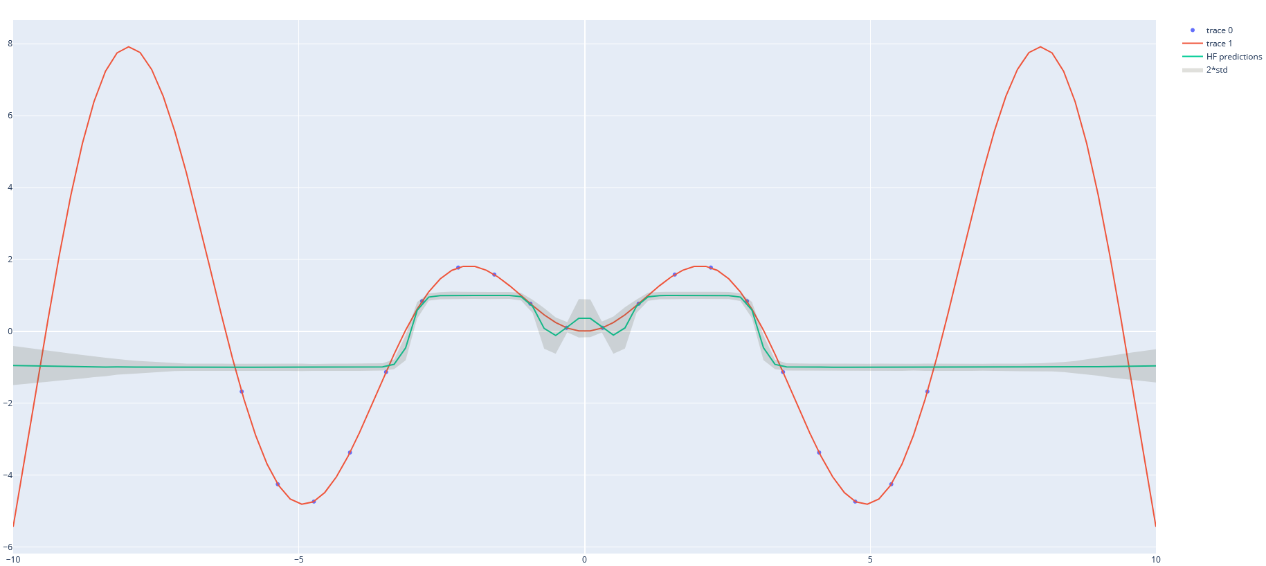
Although numpyro is much much faster, there is definitely something wrong compared to what pyro gives me, it is obvious for the MAP estimate, and less clear for the MCMC (with much less sample for pyro).

I will try next to initialize MCMC with MAP estimates. But in the meantime, any idea of what is going wrong with the numpyro model?

---

With numpyro:

With Pyro:

This is the code for numpyro for my simple test:

import jax.numpy as jnp
import jax.random as random
from jax import vmap

import numpy as np
import numpyro
from numpyro import handlers
import numpyro.distributions as distnumpyro
from numpyro.infer import MCMC as MCMCnumpyro
from numpyro.infer import NUTS as NUTSnumpyro
from numpyro.infer import Predictive as PredictiveNumpyro
import os
import time
import plotly.graph_objects as go
from collections import namedtuple


def model_bnn_numpyro(X, Y, hid_dim=5, out_dim=1, prior_scale=10.0, output_prior_scale=0.5):
    N, D_X = X.shape
    D_H = hid_dim
    D_Y = out_dim
    activation = jnp.tanh
    # sample first layer (we put unit normal priors on all weights)
    w1 = numpyro.sample("w1", distnumpyro.Normal(jnp.zeros((D_X, D_H)), jnp.ones((D_X, D_H)) * prior_scale).to_event(2))
    b1 = numpyro.sample("b1", distnumpyro.Normal(jnp.zeros(D_H), jnp.ones(D_H) * prior_scale).to_event(1))
    z1 = activation(jnp.matmul(X, w1) + b1)  # <= first layer of activations

    # sample final layer of weights and neural network output
    w3 = numpyro.sample("w3", distnumpyro.Normal(jnp.zeros((D_H, D_Y)), jnp.ones((D_H, D_Y)) * prior_scale).to_event(2))
    b3 = numpyro.sample("b3", distnumpyro.Normal(jnp.zeros(D_Y), jnp.ones(D_Y) * prior_scale).to_event(1))
    z3 = activation(jnp.matmul(z1, w3) + b3) # <= output of the neural network

    #prec_obs = numpyro.sample("prec_obs", distnumpyro.Gamma(3.0, 1.0))
    #sigma_obs = 1.0 / jnp.sqrt(prec_obs)

    # observe data
    with numpyro.plate("data", N):
        numpyro.sample("Y", distnumpyro.Normal(z3, output_prior_scale * output_prior_scale).to_event(1), obs=Y)

# helper function for HMC inference
def run_inference(model, args, rng_key, X, Y, D_H, prior_scale, output_prior_scale):
    start = time.time()
    kernel = NUTSnumpyro(model)
    mcmc = MCMCnumpyro(
        kernel,
        num_warmup=args.num_warmup,
        num_samples=args.num_samples,
        num_chains=args.num_chains,
        progress_bar=False if "NUMPYRO_SPHINXBUILD" in os.environ else True,
    )
    mcmc.run(rng_key, X, Y, D_H, prior_scale=prior_scale , output_prior_scale=output_prior_scale)
    #mcmc.print_summary()
    print("\nMCMC elapsed time:", time.time() - start)
    return mcmc.get_samples(), mcmc
    
def run_vi(model, guide, n_steps, step_size, rng_key, X, Y, D_H, prior_scale, output_prior_scale):
    adam = numpyro.optim.Adam(step_size=step_size)
    elbo = numpyro.infer.Trace_ELBO(num_particles=1)

    svi = numpyro.infer.SVI(model, guide, adam, elbo)  # optimization variable are automatically inferred from guide definition

    svi_result = svi.run(
        rng_key=rng_key, 
        num_steps=n_steps, 
        X=X, Y=Y, hid_dim=D_H,
        prior_scale=prior_scale, output_prior_scale=output_prior_scale
    )
    return svi_result

if __name__ == "__main__":
    # Generate training and test data
    x_train = np.linspace(0, 1, 20)
    x_train = x_train * 12 - 6
    y_train = x_train * np.sin(x_train)

    x_test = x_test = np.linspace(0, 1, 100)
    x_test = x_test * 20 - 10
    y_test =  x_test * np.sin(x_test)

    d_input = [
        go.Scatter(x=x_train, y=y_train, mode='markers', name='Train sample'),
        go.Scatter(x=x_test, y=y_test, mode='lines', name='True')
    ]

    N_neur = 5
    prior_scale=10.0
    output_prior_scale=0.5

    # Variational Inference: MAP
    autoguide = numpyro.infer.autoguide.AutoDelta(model_bnn_numpyro)
    svi = run_vi(
        model_bnn_numpyro, 
        autoguide,
        50000,
        1e-3,
        random.PRNGKey(1),
        x_train[:,np.newaxis],
        ( (y_train - y_train.mean()) / y_train.std() )[:,np.newaxis],
        N_neur,
        prior_scale,
        output_prior_scale
    )
    # Get samples from approximate posterior
    predictive = numpyro.infer.Predictive(model_bnn_numpyro, guide=autoguide, num_samples=2000)
    svi_samples = predictive(random.PRNGKey(1), x_test[:,np.newaxis], Y=None, hid_dim=5, prior_scale=10.0, output_prior_scale=0.5)
    samples_from_svi = svi_samples['Y'] * y_train.std() + y_train.mean()

    mean_from_svi = samples_from_svi.mean(0).squeeze()
    std_from_svi = samples_from_svi.std(0).squeeze()
    yplus_from_svi = mean_from_svi + 2*std_from_svi
    yminus_from_svi = mean_from_svi - 2*std_from_svi


    # Sample via MCMC
    rng_key, rng_key_predict = random.split(random.PRNGKey(0))
    Args = namedtuple("args", "num_warmup num_samples num_chains")
    args = Args(2000, 5000, 1)


    samples, mcmc = run_inference(
        model_bnn_numpyro,
        args, 
        rng_key,
        x_train[:,np.newaxis],
        ( (y_train - y_train.mean()) / y_train.std() )[:,np.newaxis],
        N_neur,
        prior_scale,
        output_prior_scale
    )

    # Get the posterior samples
    predictive = PredictiveNumpyro(model_bnn_numpyro, samples)
    predictions = predictive(rng_key_predict, X=x_test[:,np.newaxis], Y=None, hid_dim=N_neur)['Y'].squeeze()
    mean_prediction = jnp.mean(predictions, axis=0)
    std_prediction = jnp.std(predictions, axis=0)
    yplus = mean_prediction + 2*std_prediction
    yminus = mean_prediction - 2*std_prediction

    # Plot it
    fig = go.Figure(
        d_input + [
            go.Scatter(x=x_test, y=mean_prediction, mode='lines', name='HF MCMC predictions'),
            go.Scatter(
                x=x_test.tolist() + x_test.tolist()[::-1], # x, then x reversed
                y=yplus.tolist() + yminus.tolist()[::-1], # upper, then lower reversed
                fill='toself',
                fillcolor='rgba(100,100,80,0.2)',
                line=dict(color='rgba(255,255,255,0)'),
                hoverinfo="skip",
                showlegend=True,
                name='2*std MCMC'
            ),
            go.Scatter(x=x_test, y=mean_from_svi, mode='lines', name='HF SVI predictions'),
            go.Scatter(
                x=x_test.tolist() + x_test.tolist()[::-1], # x, then x reversed
                y=yplus_from_svi.tolist() + yminus_from_svi.tolist()[::-1], # upper, then lower reversed
                fill='toself',
                fillcolor='rgba(100,100,80,0.2)',
                line=dict(color='rgba(255,255,255,0)'),
                hoverinfo="skip",
                showlegend=True,
                name='2*std SVI'
            )
        ]
    )
    fig.write_html('numpyro_simple_bnn.html')

And the same code for Pyro:

import numpy as np
import os
import time
import plotly.graph_objects as go
from collections import namedtuple

import torch
import pyro
import pyro.distributions as dist
from pyro.nn import PyroModule, PyroSample
import torch.nn as nn
from pyro.infer import MCMC, NUTS, Predictive


class OneHiddenLayerBNN(PyroModule):
    def __init__(self, in_dim=1, out_dim=1, hid_dim=5, prior_scale=10., output_prior_scale=0.5):
        super().__init__()

        self.output_prior_scale = output_prior_scale
        
        self.activation = nn.Tanh() # or ReLU()
        self.layer1 = PyroModule[nn.Linear](in_dim, hid_dim)
        self.layer2 = PyroModule[nn.Linear](hid_dim, out_dim)

        # Set layer parameters as random variables
        self.layer1.weight = PyroSample(dist.Normal(torch.tensor(0.), prior_scale).expand([hid_dim, in_dim]).to_event(2)) # Latent random variables
        self.layer1.bias = PyroSample(dist.Normal(torch.tensor(0.,), prior_scale).expand([hid_dim]).to_event(1)) # Latent random variables
        self.layer2.weight = PyroSample(dist.Normal(torch.tensor(0.), prior_scale).expand([out_dim, hid_dim]).to_event(2)) # Latent random variables
        self.layer2.bias = PyroSample(dist.Normal(torch.tensor(0.), prior_scale).expand([out_dim]).to_event(1)) # Latent random variables

    def forward(self, x, y=None):
        x = x.reshape(-1, 1)
        x = self.activation(self.layer1(x))
        mu = self.layer2(x).squeeze()
        #sigma = pyro.sample('sigma', dist.Gamma(torch.tensor(0.5, device="cuda"), 1.0)) # Infer response noise, Latent random variables

        # Sampling model
        with pyro.plate('data', x.shape[0]):
            obs = pyro.sample('obs', dist.Normal(mu, self.output_prior_scale * self.output_prior_scale), obs=y)  # observed variable
        return mu

# helper function for HMC inference
def run_inference(model, args, X, Y):
    start = time.time()
    nuts_kernel = NUTS(model, jit_compile=True)
    mcmc = MCMC(nuts_kernel, num_samples=args.num_samples, warmup_steps=args.num_warmup)

    mcmc.run(X, Y)
    print("\nMCMC elapsed time:", time.time() - start)
    return mcmc.get_samples(), mcmc
    
def run_vi(model, guide, n_steps, step_size, X, Y):
    pyro.clear_param_store() # reinit params

    adam = pyro.optim.Adam({'lr': step_size}) # thin wrapper around pytorch adam, we could also give a function that returns parameters depending on parameter name (https://pyro.ai/examples/svi_part_i.html#Optimizers)
    elbo = pyro.infer.Trace_ELBO(num_particles=1)
    svi = pyro.infer.SVI(model, guide, adam, elbo)  # optimization variable are automatically inferred from guide definition

    losses = []

    for step in range(n_steps):
        loss = svi.step(X, Y) # takes a single gradient step and returns an estimate of the loss
        losses.append(loss)
        
        if step % 500 == 0:
            print('Elbo loss: {}'.format(loss))

    return svi

if __name__ == "__main__":
    # Generate training and test data
    x_train = np.linspace(0, 1, 20)
    x_train = x_train * 12 - 6
    y_train = x_train * np.sin(x_train)

    x_test = x_test = np.linspace(0, 1, 100)
    x_test = x_test * 20 - 10
    y_test =  x_test * np.sin(x_test)

    d_input = [
        go.Scatter(x=x_train, y=y_train, mode='markers', name='Train sample'),
        go.Scatter(x=x_test, y=y_test, mode='lines', name='True')
    ]

    torch.set_default_dtype(torch.float64)
    xt = torch.from_numpy(x_train)
    yt = torch.from_numpy(((y_train - y_train.mean()) / y_train.std()))

    N_neur = 5
    prior_scale=10.0
    output_prior_scale=0.5

    model = OneHiddenLayerBNN(hid_dim=N_neur, prior_scale=prior_scale, output_prior_scale=output_prior_scale)

    # Variational Inference: MAP
    autoguide = pyro.infer.autoguide.AutoDelta(model)
    svi = run_vi(
        model, 
        autoguide,
        50000,
        1e-3,
        xt,
        yt
    )
    # Get samples from approximate posterior
    predictive = pyro.infer.Predictive(model, guide=autoguide, num_samples=2000)
    # Second, run the model in forward using the guide samples instead of the 'a = pyro.sample('a', dist.Normal(0.0, 10.))" sample in the model
    svi_samples = predictive(x=torch.from_numpy(x_test), y=None)  # Must not provid the true y values
    samples_from_svi = svi_samples['obs'] *  y_train.std() + y_train.mean()    

    mean_from_svi = samples_from_svi.mean(0).squeeze()
    std_from_svi = samples_from_svi.std(0).squeeze()
    yplus_from_svi = mean_from_svi + 2*std_from_svi
    yminus_from_svi = mean_from_svi - 2*std_from_svi


    # Sample via MCMC
    Args = namedtuple("args", "num_warmup num_samples num_chains")
    #args = Args(2000, 5000, 1)
    args = Args(100, 500, 1)

    samples, mcmc = run_inference(
        model,
        args, 
        xt,
        yt,
    )

    # Get the posterior samples
    predictive = Predictive(model=model, posterior_samples=mcmc.get_samples())
    predictions  = predictive(x=torch.from_numpy(x_test), y=None)    
    mean_prediction = predictions['obs'].T.detach().cpu().numpy().mean(axis=1)
    std_prediction = predictions['obs'].T.detach().cpu().numpy().std(axis=1)
    yplus = mean_prediction + 2*std_prediction
    yminus = mean_prediction - 2*std_prediction

    # Plot it
    fig = go.Figure(
        d_input + [
            go.Scatter(x=x_test, y=mean_prediction, mode='lines', name='HF MCMC predictions'),
            go.Scatter(
                x=x_test.tolist() + x_test.tolist()[::-1], # x, then x reversed
                y=yplus.tolist() + yminus.tolist()[::-1], # upper, then lower reversed
                fill='toself',
                fillcolor='rgba(100,100,80,0.2)',
                line=dict(color='rgba(255,255,255,0)'),
                hoverinfo="skip",
                showlegend=True,
                name='2*std MCMC'
            ),
            go.Scatter(x=x_test, y=mean_from_svi, mode='lines', name='HF SVI predictions'),
            go.Scatter(
                x=x_test.tolist() + x_test.tolist()[::-1], # x, then x reversed
                y=yplus_from_svi.tolist() + yminus_from_svi.tolist()[::-1], # upper, then lower reversed
                fill='toself',
                fillcolor='rgba(100,100,80,0.2)',
                line=dict(color='rgba(255,255,255,0)'),
                hoverinfo="skip",
                showlegend=True,
                name='2*std SVI'
            )
        ]
    )
    fig.write_html('pyro_simple_bnn.html')