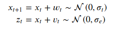
Hello,
I tried to fix the model, but still getting a bit of confusing results. The fitted local level is kind of near the true value but still it should follow the time series much closer.
Not sure what is going wrong. The data size is big 19335 rows, maybe that is the problem. Any idea what is going wrong? Appreciate any help! Thanks
model
def model(data):
    x_0 = pyro.deterministic("x_0", data[0]).unsqueeze(-1)
    sigma = pyro.sample("sigma", dist.Uniform(0, 1e-3)).unsqueeze(-1)
    w = pyro.sample("w", dist.Normal(0, 1).expand(data.shape).to_event(1))
    x_t = pyro.deterministic("x_t", x_0 + sigma * w.cumsum(dim=-1))

    sigma_z = pyro.sample("sigma_z", dist.Uniform(0, 1e-3)).unsqueeze(-1)
    z_t = pyro.sample("z_t", dist.Normal(x_t, sigma_z).expand(data.shape).to_event(1), obs=data)
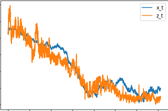
This is how the smoothed values x_t looks like
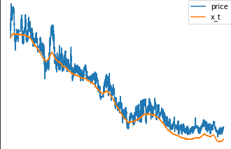
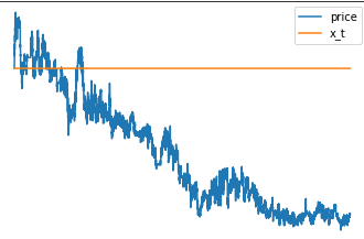
I was playing around with the model and tried to make the local level x_t only change its value in 90 % of the time. After training I got this results. Does overwriting some of the sampled values with zeros brakes the inference?
Here is the complete Code
imports
import pyro
from pyro.optim import ClippedAdam
from pyro.infer.autoguide import AutoDiagonalNormal
from pyro.infer import  SVI, Trace_ELBO, Predictive
import pandas as pd
import torch
import pyro.distributions as dist
from matplotlib import pyplot
model
def model(data):
    x_0 = pyro.deterministic("x_0", data[0]).unsqueeze(-1)
    sigma = pyro.sample("sigma", dist.Uniform(0, 1e-3)).unsqueeze(-1)
    w = pyro.sample("w", dist.Normal(0, 1).expand(data.shape).to_event(1))
    x_t = pyro.deterministic("x_t", x_0 + sigma * w.cumsum(dim=-1))

    sigma_z = pyro.sample("sigma_z", dist.Uniform(0, 1e-3)).unsqueeze(-1)
    z_t = pyro.sample("z_t", dist.Normal(x_t, sigma_z).expand(data.shape).to_event(1), obs=data)

# modified trend
def model2(data):
    x_0 = pyro.deterministic("x_0", data[0]).unsqueeze(-1)
    sigma = pyro.sample("sigma", dist.Uniform(0, 1e-3)).unsqueeze(-1)
    w = pyro.sample("w", dist.Normal(0, 1).expand(data.shape).to_event(1))
    threshold = torch.min(torch.topk(w, int(data.shape[0]*0.1)).values)
    w_new = torch.nn.functional.relu(w-threshold)
    x_t = pyro.deterministic("x_t", x_0 + sigma * w_new.cumsum(dim=-1))

    sigma_z = pyro.sample("sigma_z", dist.Uniform(0, 1e-3)).unsqueeze(-1)
    z_t = pyro.sample("z_t", dist.Normal(x_t, sigma_z).expand(data.shape).to_event(1), obs=data)
Data
df = pd.read_csv(
    'https://s3.eu-central-1.amazonaws.com/mira.collector/data.csv',
    index_col=0)
r = torch.tensor(df.price)
Training
pyro.clear_param_store()
pyro.set_rng_seed(1234567890)
num_steps = 1001
optim = ClippedAdam({"lr": 0.05, "betas": (0.9, 0.99), "lrd": 0.1 ** (1 / num_steps)})
guide = AutoDiagonalNormal(model)
svi = SVI(model, guide, optim, Trace_ELBO())
losses = []

for step in range(num_steps):
    loss = svi.step(r)
    losses.append(loss)
    if step % 50 == 0:
        median = guide.median()
        print("step {} loss = {:0.6g}".format(step, loss))
pyplot.figure(figsize=(9, 3))
pyplot.plot(losses)
pyplot.ylabel("loss")
pyplot.xlabel("SVI step")
pyplot.xlim(0, len(losses))
pyplot.ylim(min(losses), 20)
Smoothing
# We will pull out median log returns using the autoguide's .median() and poutines.
with torch.no_grad():
    pred = Predictive(model, guide=guide, num_samples=100, parallel=False)(r)
x_t = torch.mean(pred['x_t'],axis=0)
df_pred =  pd.DataFrame(x_t.numpy().squeeze(),df.index,columns=['x_t'])

pd.concat([df.price, df_pred.x_t], axis=1).plot()