Simple 1D dynamical model - uncertainty not growing during occlusion

Hello, I am implementing a standard and simple dynamical state space model of the form

image

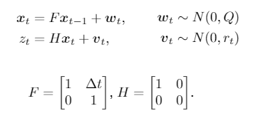
where my state x_t contains the position variable x and its velocity variable v of an unknown object. We only observe the position variable x of the object and this observation is denoted by z_t. I want to capture this behaviour in the model and infer latent variables x_t using the SVI method.

There is one twist. During some time interval, the measurements are unavailable. My goal is that the inference procedure is still able to infer these unobserved states using the model structure. (This occluded interval does not have to be at the end, so I am not interested in forecasting).

I created the following implementation for 50 time steps , where one time step is of size 1. There are no measurements from time step 30 up until 50. So the last 20 time steps.

# Model
def model(prior, F, Q, r, data):
    P0 = torch.eye(prior.shape[0])
    prev_state = pyro.sample("prior", dist.MultivariateNormal(prior, P0))
    
    for t in pyro.markov(range(0,len(data))):
        # Transition model formula
        state = pyro.sample("state_{}".format(t), dist.MultivariateNormal(prev_state, Q))
        
        # Nonlinearity function h(x_t)
        c_state = state[0]
            
        # Occlusion
        r_t = r
        if t >= occ_start and t<=occ_start+occ_dur:
            r_t=10000000000.  
        
        # Observation model formula
        pyro.sample("measurement_{}".format(t), dist.Normal(c_state, r_t), obs = data[t])
        prev_state = F@state.T

I implemented two separate mean field guides that behave similarly. The first one considers 50 separate latent states and their 50 corresponding covariance matrices.
The second one combines these 50 states into one large state latent mean and one big corresponding covariance matrix.

# Guide 1
def guide(prior, F, Q, r, data):
    P0 = torch.eye(prior.shape[0])
    prev_state = pyro.sample("prior", dist.MultivariateNormal(prior, P0))
    
#     prev_state = torch.tensor([0.1,0.1])
    
    for t in pyro.markov(range(0,len(data))):
        # Mean and covariance parameters
        x_value = pyro.param("x_value_{}".format(t), torch.zeros(prior.shape[0]))
        var_value = pyro.param("var_value_{}".format(t), P0, 
                               constraint=dist.constraints.lower_cholesky)
        
        # x_t = N(x_value, var_value)
        state =  pyro.sample("state_{}".format(t), dist.MultivariateNormal(x_value, scale_tril=var_value))

And the second guide:

# Guide, with big combined multivariate distribution
def guide(prior, F, Q, r, data):
    P0 = torch.eye(prior.shape[0])
    n = prior.shape[0] # Equal to 2
    prev_state = pyro.sample("prior", dist.MultivariateNormal(prior, P0))
        
    loc = pyro.param("loc", Variable(2.0*torch.ones(prior.shape[0]*data.shape[0]), requires_grad=True))
    scale = pyro.param("scale_tril", Variable(5.0*torch.eye(prior.shape[0]*data.shape[0]), requires_grad=True), 
                           constraint=dist.constraints.lower_cholesky)     
 
    for t in pyro.markov(range(0,len(data))):
        # Mean and covariance parameters
        x_value = loc[t*n:t*n+n]
        var_value = scale[t*n: t*n + n, t*n: t*n + n] 
        
        # x_t = N(x_value, var_value)
        state =  pyro.sample("state_{}".format(t), dist.MultivariateNormal(x_value, scale_tril=var_value))

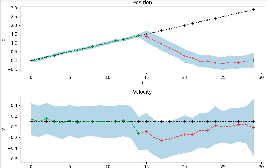
These both give similar results like this

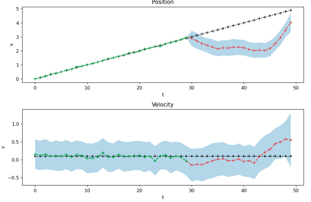
The problem here is that the estimates of the confidence bounds do not behave as expected. When you do not get new measurements anymore, you would expect that the inference procedure becomes more uncertain about its prediction every time step. Therefore I would expect the uncertainty and therefore the confidence bounds to grow if you receive no measurements at the end.
This is not the case. How can I fix this?

I was thinking about using a structured guide, but a proper mean field guide should still be able to incorporate the time dependencies of the states at different time steps.

Side note: I implemented this occlusion of measurements by drastically increasing the variance of the measurement during this interval. I specifically did not use obs_mask since, if I increase this to more dimensions and to a non-linear variant I do not want my entire measurement to be unobserved but only part of it.

Your two guides behave similarly because they are basically equivalent. As discussed in our list of SVI tips and tricks, there are a number of reasons your results could be poor, including guide parameter initialization, the mean-field assumption, insufficient optimization for convergence, or model parametrization.

However, keep in mind that writing and working with custom guides can be tricky, so you might try using an autoguide like AutoMultivariateNormal or AutoLowRankMultivariateNormal if you are interested in a non-mean-field approximation or AutoNormal for a mean-field approximation. If you can’t get results that are compatible with your qualitative expectations using a non-mean-field autoguide, it’s likely that the problem is with your model, data or optimization setup.

since you’re using an explicit for loop i would suggest you model occlusion as

pyro.sample("measurement_{}".format(t), dist.Normal(c_state, r_t), obs = None)

you will then need to introduce corresponding sample sites in the guide for the missing observations. this may give you better results. baking in numbers like 10000000000 may lead to bad numerics

Thank you for your responses.

@eb8680_2 I tried several auto guides as well. The AutoNormal guide gave the same results (since I am not showing the covariance estimates between the position and velocity states). The AutoMultivariateNormal guide does not train succesfully, after around 5 SVI steps, I get NaNs in my scale parameter. I tried changing the initialization parameters but that did not seem to work. However, I expect that this guide would be similar to my second guide that I have shown above, so I would expect similar results.

Therefore, this does unfortunately not help in finding the exact problem that is, why Pyro is not taking into account the time dependency between states and therefore the dependency between covariances. Do you maybe have additional suggestions about what I can try? E.g. how to code this time dependency explicitely for example.

@martinjankowiak I implemented the different occlusion approach using obs=None as well. As expected, this gave the exact same results as before. (It did not solve the NaN issue for the AutoMultivariateNormal guide.)
Question: In the scenario of a multivariate observation, is it possible to only occlude one part of the observation using the obs=None or obs_mask statements? So for example, if you have observation Z = (z1,z2), can you specify that only z1 is observed for a specific time interval, but z2 is not? If not, then I think using my previous approach where I increase the variance drastically would be the only solution.

i don’t know why you can’t get it to work. for example i have no idea what the scale of your data is.

i suggest you:

  • use fewer time steps and see if you can get it to work in that regime
  • avoid high-dimensional multivariate normal distributions in your guide
  • initialize x_value at raw observation when available
  • initialize your guide variances to something much smaller, e.g.
        var_value = pyro.param("var_value_{}".format(t), 0.01 * P0, 
                               constraint=dist.constraints.lower_cholesky)

After tweaking some parameters and decreasing the number of steps and decreasing the learning rate, I got the AutoMultivariateNormal guide to work as well. This one gave similar results as before. For more information about the scale of my data, I currently use these settings.

# Initial paramters
NUM_STEPS = 30  
delta_t = 1.0  
F=torch.tensor([[1, delta_t],[0, 1]])
# Occlusion start and duration
occ_start = 15
occ_dur = 15

## Data Simulation
# Latent states
data_v = torch.zeros(NUM_STEPS, 2)
data_v[0] = torch.tensor([0., 0.1])
for i in range(1,NUM_STEPS):
    data_v[i] = F@data_v[i-1]
    
# Observations
c_obs_v = torch.zeros(len(data_v))
for i in range(len(data_v)):
    c_obs_v[i] = data_v[i,0] + 0.03 * randn()

# Model parameters
prior = torch.tensor([0.0,0.3])  
Q = 0.2 * torch.eye(2)
Q[1,1] = 0.3
r = 0.1

It is not the case that something is not working. The inference procedure is training correctly and I do get results. They are however not the results I would expect.

Once occlusion occurs, I would expect that it uses the model to make predictions of the next time step using the previous time step. The further in time these predictions are without any feedback of the observations, the bigger I expect the confidence bounds to be.

Clearly this is not happening. There does not seem to be dependencies in the variance on previous time steps at all.
Right now I don’t exactly know what causes this. Could this for example be due to the limitations of my simple guide? Or is Pyro simply not designed to take the dependencies of the trained parameters on other time steps into account.

in principle pyro can fit any parametric variational distribution (guide) to a model. the thing is that doing so properly requires solving a stochastic optimization problem. in general this problem can be arbitrarily hard. did you try making the problem easier?

for example:

NUM_STEPS = 10  
occ_start = 7
occ_dur = 3

by making the problem easier it can be easier to identify optimization difficulties. for example, what if you initialize your guide to look like the answer you expect?

note that variational inference isn’t always a great fit for these kinds of time series problem, especially one with so much missingness. you’d probably get better results using HMC.

Yes when I did try to make the problem smaller and easier and the estimates did seem to converge better. When I initialize the guide to the correct positions and growing covariance, it diminishes this growing covariance to a constant one, but keeps the positions at the initialized and correct points.

At the end I still didn’t figure out why the confidence bounds stay the same over time. Maybe this has something to do with the fact that SVI tends to understimate the covariance?

I do have an alternative question regarding my implementation. Do you think my model correctly captures the dynamics that I showed using the dynamic formulas from my original post?
The reason I am asking this is because I could not really find comparable models online and I noticed some interesting behaviour:
In the predictions of the position estimate during occlusion, it does not seem to take the transition from the previous time step x_t = F x_(t-1) into account, so I was wondering if I correctly captured this transition in the model or not.
Instead during occlusion it sticks to the guide initialization that in my original figure was set to 2.0 and in the second figure set to 0.0. However, I would expect that it would rely on the model more during occlusion and use the transition p_t = p_(t-1) + \delta_t * v_(t-1) as a position prediction. This one should point the next position estimate upwards because of the big velocity initialization and not downwards as in the figure…

Additionally I would like one of my previous questions again

Question: In the scenario of a multivariate observation, is it possible to only occlude one part of the observation using the obs=None or obs_mask statements? So for example, if you have observation Z = (z1,z2), can you specify that only z1 is observed for a specific time interval, but z2 is not? If not, then I think using my previous approach where I increase the variance drastically would be the only solution.

At the end I still didn’t figure out why the confidence bounds stay the same over time. Maybe this has something to do with the fact that SVI tends to understimate the covariance?

yes probably part of what’s going on. this can be especially exasperated when you make mean field assumptions (factorized variational distribution)

Do you think my model correctly captures the dynamics that I showed using the dynamic formulas from my original post?

i don’t have the time to look at your model code in granular detail but it seemed ok to me

you could certainly try a guide where the variational mean for state_t is regressed against the sampled state_{t-1}. this would be more flexible

the best way to do something like this would be to build a custom distribution that allows such masking. a construct like pyro.poutine.mask does not allow you to “peer into” an arbitrary multivariate distribution; rather it allows you to mask entire “events” one at a time

Thank you so much for your response! I have one final question.

you could certainly try a guide where the variational mean for state_t is regressed against the sampled state_{t-1} . this would be more flexible

How could I acchieve something like this? I don’t have a good idea yet how to apply this idea in the guide using the Pyro syntax.

a guide is just a python function that contains various sample and param statements nothing exotic is needed to include more complex dependency structure.

something vaguely like this:

def guide(prior, F, Q, r, data):
    P0 = torch.eye(prior.shape[0])
    # note this isn't great because you're fixing the guide to the prior at the first time step
    prev_state = pyro.sample("prior", dist.MultivariateNormal(prior, P0))

    for t in pyro.markov(range(0,len(data))):
        F_t = pyro.param("F_{}".format(t), F)
        x_value = pyro.param("x_value_{}".format(t), torch.zeros(prior.shape[0]))
        var_value = pyro.param("var_value_{}".format(t), P0, 
                               constraint=dist.constraints.lower_cholesky)
        
        prev_state = pyro.sample("state_{}".format(t), dist.MultivariateNormal(x_value + F_t @ prev_state, scale_tril=var_value))