Scale of Normal posterior stays constant despite increasing the number of observed data points

Hello!

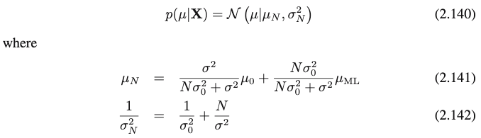
I’m toying with one of simplest examples involving Bayesian inference: modeling 1-dimensional data x using a Gaussian distribution N(x | μ, σ²) with prior over the mean N(μ | μ₀, σ₀²) and fixed variance

def model(x):
    m0 = torch.tensor(0.0)
    s0 = torch.tensor(10.0)

    m = pyro.sample("m", dist.Normal(m0, s0))
    s = torch.tensor(1.0)

    pyro.sample("x", dist.Normal(m, s), obs=torch.tensor(x))

The posterior of the mean is set to a Gaussian distribution p(μ | x) ≅ q(μ) = N(μ | μ_q, σ²_q) by using the AutoNormal guide.

When training on a large synthetic dataset, the mean of the posterior μ_q does converge to the true mean of the data, but the variance σ²_q seems to stay constant – I was expecting it to decrease to 0 as more evidence is gathered.

...
  900 |   +3.068 | AutoNormal.locs.m:   2.98, AutoNormal.scales.m:   0.99
  950 |   +6.529 | AutoNormal.locs.m:   2.99, AutoNormal.scales.m:   1.04
 1000 |   +3.376 | AutoNormal.locs.m:   2.93, AutoNormal.scales.m:   1.09
 1050 |   +3.509 | AutoNormal.locs.m:   2.99, AutoNormal.scales.m:   1.08
 1100 |   +4.299 | AutoNormal.locs.m:   2.97, AutoNormal.scales.m:   1.13
...

Any ideas of what might be happening? I’m surely missing something fundamental, so any guidance is appreciated.

Here is the complete code:

import torch
import numpy as np

import pyro
import pyro.distributions as dist

from pyro.infer import SVI, Trace_ELBO
from pyro.infer.autoguide import guides
from pyro.optim import Adam


SEED = 1337
np.random.seed(SEED)
pyro.enable_validation(True)


def load_data(num_points, mu, sigma):
    x = np.random.randn(num_points)
    return mu + sigma * x


def model(x):
    m0 = torch.tensor(0.0)
    s0 = torch.tensor(10.0)

    m = pyro.sample("m", dist.Normal(m0, s0))
    s = torch.tensor(1.0)

    pyro.sample("x", dist.Normal(m, s), obs=torch.tensor(x))


guide = guides.AutoNormal(model)
optimizer = Adam({"lr": 0.01})
svi = SVI(model, guide, optimizer, loss=Trace_ELBO())

data = load_data(5000, 3, 1)
fmt = lambda p: ", ".join(f"{k}: {v.item():6.2f}" for k, v in p.items())

for it, x in enumerate(data):
    nll = svi.step(x)
    if it % 50 == 0:
        params = pyro.get_param_store()
        print(f"{it:5d} | {nll:+8.3f} |", fmt(params))


params = pyro.get_param_store()
print("estimated:  ", fmt(params))

Hi, I believe the model is correct and your expectation is wrong. If you carefully look at how you created your data, you see that your data actually has the unit variance (Please note that np.random.randn(num_points) generate data points with 0 mean 1 std). Once you add mu, the variance stay the same as 1. Therefore, your model’s prediction of scale as 1 should be correct.

Thank you for the answer @yilmazcanozyurt! I understand that the data has unit variance, but I don’t see why the posterior of the mean should also have unit variance. Concretely, in Pattern Recognition and Machine Learning (section 2.3.6), the author computes analytically the posterior and its variance is inversely proportional to the number of observed points N:
image
The author also mentions:

[I]f the number of data points N → ∞ , the variance σ²_N goes to zero and the posterior distribution becomes infinitely peak around the maximum likelihood solution.

Edit: Maybe the inconsistency appears because I’m iterating through the points one by one, instead of using batches of N points?

yes you need to use pyro.plate so that subsampling is taken into account properly. for example see this tutorial

1 Like

Thanks a lot for the clarification @martinjankowiak! Indeed, if I (i) use plate with subsample_size=1 and (ii) pass the entire dataset to the model, then I do obtain the desired variance for the posterior. (I’m still not sure what the semantics of the initial code was.)

A couple of related questions:

  • How does one update the posterior sequentially (or on-line, that is, data points come one at a time and we don’t have access to the entire dataset at once)?

  • In the initial code, I would have expected m0 and s0 to represent the prior over the mean m,
    but judging by the values of AutoNormal.locs.m and AutoNormal.scales.m at the first iterations, it seems they start from 0 and 0.1, respectively, regardless of how I set m0 and s0.
    Edit: I see in the documentation that AutoNormal assumes a standard Normal distribution, N(0, 1) – although init_scale defaults to 0.1, and not to 1. I assume that the values in the model m0 and s0 are ignored, right?

  • there is no generic way to do online bayesian inference. unless one is dealing with a very particular (conjugate) model, this sort of thing invariably involves approximations.

  • if i understand your second question: no, AutoNormal does not inspect the details (e.g. the mean parameters) of the model prior distributions when initializing its variational parameters

1 Like

I assume I could do online Bayesian inference by sequentially updating the prior based on the posterior computed on the last data point. This approach is certainly inefficient and not idiomatic, but are there any other issues with it? Does this work only for conjugate distributions? :thinking:

I see there are some papers on online (sequential) variational inference, but I haven’t studied them properly to see if their ideas can be ported to Pyro (e.g., Streaming Variational Bayes from Michael I. Jordan’s group).

Yes, sorry, my thoughts were just muddled; I think it is clearer now.

Thanks again for the explanations!

Dan.

you can certainly do online variational inference for certain kinds of models using a computational flow in which you continuously replace the prior with your latest posterior approximation. this is all fine and good but in the general case it’s an approximation, i.e. you’re always losing information about some of the data you’re not revisiting (since your approximate posterior never recovers the exact posterior)

1 Like