RuntimeError: Cannot find valid initial parameters. Please check your model again

Dear All,

I know this must be a stupid bug, but I cannot find what triggers this issue. I have a Planck black body radiation model that should be relatively straightforward to sample.

import jax.numpy as jnp
import jax

@jax.jit
def bb_flux(
    λnm: "nanometers", 
    T: "K",
    amp: float = 1.) -> jnp.array:
    """
    default units blackbody as a flux distribution as a function of wavelength,
    temperature and amplitude.
    
    :param lam:   wavelength in nm
    :param amp:   dimensionless normalization factor
    :param teff: temperature in Kelvins
    :return: evaluation of the blackbody radiation in flam units (erg/s/cm2/AA)
    """
    # Constants
    h = 6.626e-34 # Planck's constant [J*s = m**2 * kg / s]
    c = 2.998e8 # Speed of light [m/s]
    k = 1.381e-23 # Boltzmann constant [J/K]

    # Planck's law
    λ = λnm * 1e-9
    return amp * 2 * h * c ** 2/ (λ ** 5 * (jnp.exp(h * c/(λ * k * T)) - 1))

The following is one of the attempts to describe the model.

import numpyro
import numpyro.distributions as dist

def model(λm: jnp.array, 
          fobs: jnp.array = None):
    """ Model of the fobs | fpred, λ, ω """

    T = numpyro.sample('T', dist.Uniform(3000., 10000.))
    log_amp = numpyro.sample('log_amp', dist.Uniform(-0.01, 0.01))
    amp = jnp.power(10., log_amp)
    fhat = numpyro.deterministic('fhat', bb_flux(λnm, T, amp))
    residuals = jnp.nan_to_num(fobs - fhat)
    numpyro.factor('obs', dist.Normal(0, 1e4).log_prob(residuals).sum())

In this model, the factor could be replaced by numpyro.sample('obs', dist.normal(fhat, 1e4), obs=fobs).
(the issue remains)

The inference does not run because of an initialization error

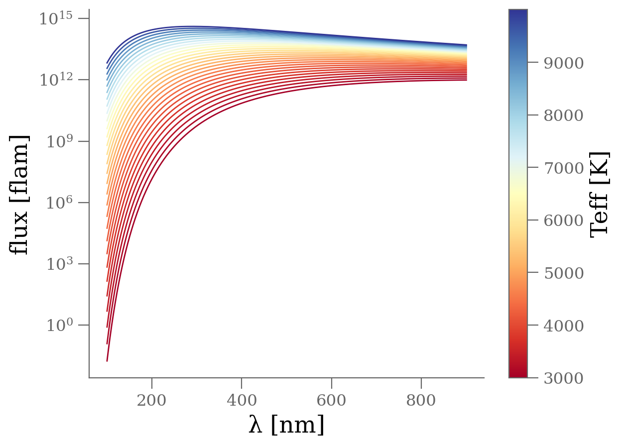
λnm = np.linspace(100, 900, 1000)
teff_true = 4500  # _K
amp_true = 1.
fobs = amp_true * bb_flux(λnm, teff_true, amp_true)

from numpyro import infer
kernel = infer.NUTS(model, init_strategy=infer.init_to_median())
sampler = infer.MCMC(
    kernel,
    num_chains=1, num_warmup=1000, num_samples=2000, 
    progress_bar=True)
sampler.run(jax.random.PRNGKey(7), λnm, fobs)

RuntimeError: Cannot find valid initial parameters. Please check your model again.

I tried the init_strategy keyword but could not make this change anything.

Does anyone see the obvious mistake? I suspect it comes from the numerical dynamics of the bb_flux outputs, but there must be something to do, right?

i don’t know what’s going on but i’d suggest revising units so that everything is O(1) so e.g. T is O(1) instead of O(10^4)

But there is no issue evaluating the model and log_prob of the model. So I do not really understand what creates the issue.

hmc uses gradients to explore a log density surface. the scale of the surface in different directions matters. if the coordinates are such that O(1) moves in each direction result in O(1) changes in log density it’s more likely that default settings of e.g. the mass matrix are reasonable. evaluating a density at a fixed point is much easier than exploring a density in a neighborhood.

ok but I have no idea of the transformation that would help here. The quantities have huge dynamics.

i don’t know either but try by using e.g. units of 1000 kelvin

Thanks. Indeed, I managed by changing the internal units

For completeness below is a functional solution

@jax.jit
def bb_flux(λnm, T) -> jnp.array:
    """
    Compute the Black Body Planck function given wavelength and Temperature

    This function internally works in cgs to help the nmerical performance.

    :param λnm:   wavelength in nm
    :param T:     temperature in Kelvins
    :return:      evaluation of the blackbody radiation in flam units / steradians 
    """
    # Constants
    # Declare global constants with numeric values to allow for relatively
    # high-performance (low-overhead) with appropriate units (cgs here)
    h = 6.62607015e-27 # Planck's constant  [erg s]
    c = 29979245800.0  # Speed of light     [cm / s]
    k = 1.380649e-16   # Boltzmann constant [erg / K]
    λcm = λnm * 1e-7
    I = (2 * h * c ** 2 / λcm ** 5 * (jnp.exp( h * c / ( k * T * λcm)) - 1) ** -1)
    # I in  erg/s/cm**2/cm/sr
    return I * 1e-8 # to flam / sr


def model(λnm: jnp.array, 
          fobs: jnp.array = None,
          ferr: jnp.array = None):
    """ Model of the fobs | fpred, ferr, λ
    
    :param λnm:  wavelengthd in nm 
    :param fobs: observed SED at λnm
    :param ferr: uncertainties on SED
    """

    T = numpyro.sample('T', dist.Uniform(3000, 10000))
    log_amp = numpyro.sample('log_amp', dist.Uniform(-2, 2))
    amp = jnp.power(10., log_amp)
    fhat = numpyro.deterministic('fhat', amp * bb_flux(λnm, T))

    if ferr is None:
        ferr = 0.1 * fhat
    
    n = len(λnm)
    with numpyro.plate(f"λ=0..{n:,d}", n): 
        numpyro.sample('fpred', dist.Normal(fhat, ferr), obs=fobs)