I am trying to create regression with exponential distributed errors.
I am trying to estimate the regression like this
import numpy as np
import numpyro
from numpyro import distributions as dist
from numpyro.infer import MCMC, NUTS
import jax
import jax.numpy as jnp
numpyro.set_host_device_count(2)
import matplotlib.pyplot as plt
a = 2
b = 2
lam = 1/2
x_data = np.random.uniform(-2, 2, 100)
y_data = a + b * x_data + np.random.exponential(lam, x_data.size)
def model1(x=None, y=None):
a = numpyro.sample("a", dist.Uniform(1.0, 3.0))
lam = numpyro.sample("lambda", dist.Exponential(1))
M = 0.0
if x is not None:
bM = numpyro.sample("b", dist.Uniform(0.0, 4.0))
M = bM * x
mu = numpyro.deterministic("mu", a + M, )
ExponentialShift = dist.TransformedDistribution(
dist.Exponential(rate=lam),
dist.transforms.AffineTransform(mu, 1),
)
with numpyro.plate("data", len(x)):
numpyro.sample("obs", ExponentialShift, obs=y)
# Using the model above, we can now sample from the posterior distribution using the No
# U-Turn Sampler (NUTS).
sampler1 = MCMC(
NUTS(model1),
num_warmup=3000,
num_samples=10000,
num_chains=2,
progress_bar=True,
)
sampler1.run(jax.random.PRNGKey(0), x_data, y=y_data)
summary = sampler1.get_samples()
a_hat = summary["a"].mean()
b_hat = summary["b"].mean()
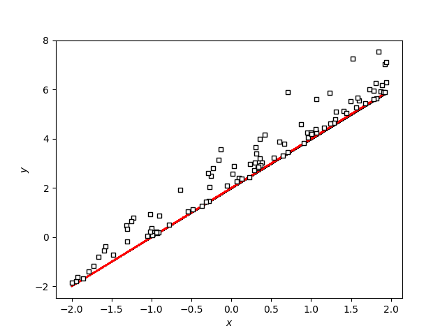
plt.scatter(x_data, y_data, marker="s", s=22, c="w", edgecolor="k", zorder=1000)
plt.plot(x_data, (a_hat + b_hat * x_data), color="k", lw=1.5)
plt.plot(x_data, a + b * x_data, color = "r")
plt.xlabel("$x$")
plt.ylabel("$y$")
plt.show()
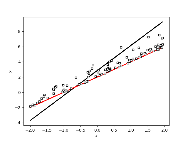
I think the problem is that I am applying the AffineTransform incorrectly since when I modify my example like that it seems to work
def model2(x, y):
a = numpyro.sample('a', dist.Normal(0, 10))
b = numpyro.sample('b', dist.Normal(0, 10))
lambda_err = numpyro.sample('lambda', dist.Exponential(1.0))
mean = a + b * x
err = numpyro.sample('err', dist.Exponential(lambda_err), sample_shape=(len(x),))
numpyro.sample('y', dist.Normal(mean + err, .001), obs=y)
# Using the model above, we can now sample from the posterior distribution using the No
# U-Turn Sampler (NUTS).
sampler2 = MCMC(
NUTS(model2),
num_warmup=3000,
num_samples=10000,
num_chains=2,
progress_bar=True,
)
sampler2.run(jax.random.PRNGKey(0), x_data, y=y_data)
summary = sampler2.get_samples()
a_hat = summary["a"].mean()
b_hat = summary["b"].mean()
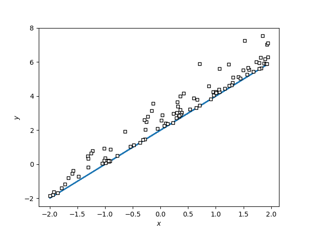
plt.scatter(x_data, y_data, marker="s", s=22, c="w", edgecolor="k", zorder=1000)
plt.plot(x_data, (a_hat + b_hat * x_data), color="k", lw=1.5)
plt.plot(x_data, a + b * x_data, color = "r")
plt.xlabel("$x$")
plt.ylabel("$y$")
plt.show()