I am playing around with autoguides in SVI, and am trying to extract the constrained domain covariance matrix from a successful MultivariateNormal autoguide. I am getting the correct distribution / covariance when drawing samples from the resulting posterior using Predict, but haven’t been able to find the most elegant way to get the raw covariance matrix from which these samples are being drawn.
E.g.:
# ------------------------
# Model
sig1, sig2, theta = 2.0, 5.0, 45*np.pi/180 # True params

def model_forauto():
    x = numpyro.sample('x', dist.Uniform( -10 , 10))
    y = numpyro.sample('y', dist.Uniform( -10 , 10))

    c,s = jnp.cos(theta), jnp.sin(theta)
    log_fac = -1.0 / 2.0 * ( ( (c*x- s*y) / sig1 )**2 + ( (s*x + c*y) / sig2)**2 )
    numpyro.factor('logfac', log_fac)

# ------------------------
# SVI Work
optimizer_forauto = numpyro.optim.Adam(step_size=0.0005)

autoguide = numpyro.infer.autoguide.AutoMultivariateNormal(model_forauto)

autosvi = SVI(model_forauto, autoguide, optim = optimizer_forauto, loss=Trace_ELBO())
autosvi_result = autosvi.run(random.PRNGKey(1), 50000)

# ------------------------
# Recover Covariance Matrix
L = autosvi_result.params["auto_scale_tril"]
COVAR_REC = jnp.dot(L,L.T)
Doing things this way, I get a covariance matrix with the correct ‘shape’, but multiplied by a factor that changes with prior width, distribution width etc. e.g. for the above, the correct covariance matrix should be:
But I am recovering something that is too small by a factor of ~23.33
I’ve tried various attempts to transform back manually using autoguide.get_transform(params = autosvi_result.params) and its various properties (e.g. the Jacobian determinant) but haven’t found a clear way to recover the scale that generalizes to all cases.
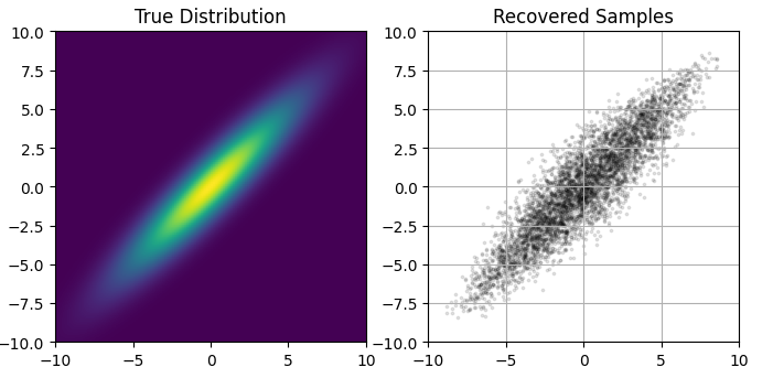
To confirm that the SVI itself is converging correctly, here is a comparison of the true likelihood function (left) to the samples recovered from Predictive(autoguide, params=autosvi_result.params, num_samples=5000)