Potential Bug in GaussianHMM - Ambiguous cause, but clear example

Hey guys - apologies for all the posts, but I am again running into some strange behavior with the GaussianHMM. I noticed some odd results that i was seeing, and ran this simulation - a simple 2-d random walk GaussianHMM:

import numpy as np
import matplotlib.pyplot as plt
import torch
import pyro
import pyro.distributions as dist
from torch.distributions import constraints
from pyro import poutine

pyro.set_rng_seed(1)

obs = torch.eye(2)
init_dist = dist.Normal(torch.zeros(2),1.).to_event(1)
transition = torch.eye(2)
transition_dist = dist.Normal(torch.zeros(2),1).to_event(1)
obs_dist = dist.Normal(torch.zeros(2),.01).to_event(1)

distt = dist.GaussianHMM(init_dist, transition, transition_dist, obs, obs_dist, duration=1000000)
  
sample = distt.rsample().detach()
x =sample[:,0]
y=sample[:,1]
t = np.linspace(1, 1000000, 1000000)
plt.figure(figsize=(10, 6))
plt.plot(t, y, label='y(t)')
plt.plot(t, x, label='X(t)')
plt.xlabel('Time')
plt.ylabel('Value')
plt.legend()
plt.grid(True)
plt.show()

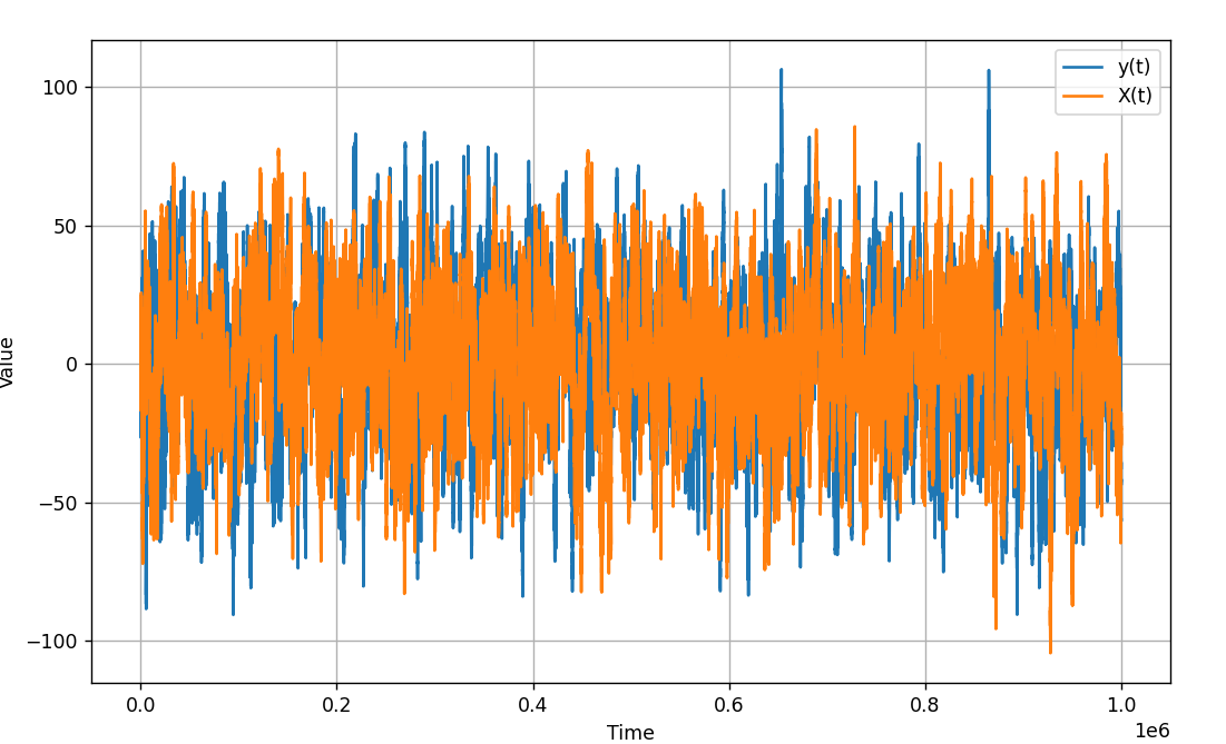
Again, this is a simple 2-d random walk (shown as y and X in the image). After running 1 million steps, I got the following graph, which is clearly not a random walk, but rather looks stationary (see image below). This makes me think there is a bug in the distribution.

The bug appears to be related to numerical precision. In this particular example, the sampling is fine for around 1000 steps or less. However, once you get to 10,000 steps and beyond, it is clear there are numerical issues.

One can see this by observing the covariance matrix:

In the method sequential_gaussian_filter_sample, we have the following code:

   gaussian = trans
    while gaussian.batch_shape[-1] > 1:
        time = gaussian.batch_shape[-1]
        even_time = time // 2 * 2
        even_part = gaussian[..., :even_time]
        x_y = even_part.reshape(shape + (even_time // 2, 2))
        x, y = x_y[..., 0], x_y[..., 1]
        x = x.event_pad(right=state_dim)
        y = y.event_pad(left=state_dim)
        joint = (x + y).event_permute(perm)
        tape.append(joint)
        contracted = joint.marginalize(left=state_dim)
        if time > even_time:
            contracted = Gaussian.cat((contracted, gaussian[..., -1:]), dim=-1)
        gaussian = contracted
    gaussian = gaussian[..., 0] + init.event_pad(right=state_dim)

one can put a breakpoint and observe the covariance matrix of gaussian, which contains the precision (and hence covariance matrix) between the initial distribution and the final data point.

In this particular example, the variance of the Nth sample point should be N+1, so for 10,000 steps, it should be 10,001. However, when setting the sample size to 10,000, the variance is between 5000 and 6000. This is clearly a bug (due to numerical issues, since performance is fine for smaller sample sizes).

Eventually, for larger sample sizes, the variance stops increasing - it hits an asymptotic max value of a variance of less than 10,000. Again, this is likely due to numerical issues.

doesn’t look like you’re using double precision?

@martinjankowiak Correct. I just noticed this myself. Switching to torch.float64 does appear to fix the issue. This was unexpected. I wasn’t expecting performance to deteriorate so quickly with float32.

generally speaking i’d recommend using double precision for all non-trivial linear algebra unless you’re not willing to pay the additional compute cost

@martinjankowiak it turns out that, even with torch.float64, the gaussianHMM will fail if the model is locally linear (which I am interested in). Here is an example that shows this is the case (the local-linear factor, the second state dimension, has transition variance very small to mimic local linear behavior). If you run the code with N=100, you’ll see everything looks fine. However, if you increase N to 10,000, the numerical precision again becomes an issue and you no longer get reasonable results (the samples are all stationary, which is incorrect. the sample should be a local-linear random walk):

import numpy as np
import matplotlib.pyplot as plt
import torch
import pyro
import pyro.distributions as dist
from torch.distributions import constraints
from pyro import poutine

pyro.set_rng_seed(1)
torch.set_default_dtype(torch.float64)
dim = 2
N = 10000
dt = 0.2

obs = torch.eye(dim)
init_dist = dist.Normal(torch.zeros(dim),1.).to_event(1)
transition = torch.tensor([[1.,0.],[dt,1.]]).transpose(0,1)
transition_dist = dist.Normal(torch.zeros(dim),torch.tensor([1.,.000001])).to_event(1)
obs_dist = dist.Normal(torch.zeros(dim),.01).to_event(1)

distt = dist.GaussianHMM(init_dist, transition, transition_dist, obs, obs_dist, duration=N)
  
sample = distt.rsample().detach()
#x =sample[:,0]
y=sample[:,1]
t = np.linspace(1, N, N)
plt.figure(figsize=(10, 6))
plt.plot(t, y, label='y(t)')
#plt.plot(t, x, label='X(t)')
plt.xlabel('Time')
plt.ylabel('Value')
plt.legend()
plt.grid(True)
plt.show()

don’t really understand what you’re trying to accomplish and it’s a long time since i looked at the relevant math but when i implemented GP-like models using GaussianHMM the stationary kernels never had vanishing variance anywhere

@martinjankowiak thanks for sharing, and looking at! I’ll see if I can work with a higher variance. the use case would be smooth local-linear models, common in financial and economic applications.