Hello! I am relatively new to Pyro, probabilistic modelling in general really. I apologise in advance that this is a long-winded problem, but I suspect it is only solvable with sufficient context.
TLDR!
Goal: Learn the parameters of a decaying sum of sine signals with added noise using Pyro’s SVI.
Problems: Noise over estimated, amplitudes under estimated, difficulty assuring parsimony, suspected bimodality in my distributions.
What I’d like help with:
- Choosing distributions / transformations for my model and guide that break the the amplitude-phase and frequency-phase degeneracies whilst encouraging unused components to go to zero.
- Wrapping my phase distribution to a domain [0, 2pi) or [-pi, pi). From what I’ve understood VonMises is incompatible with gradient optimisation.
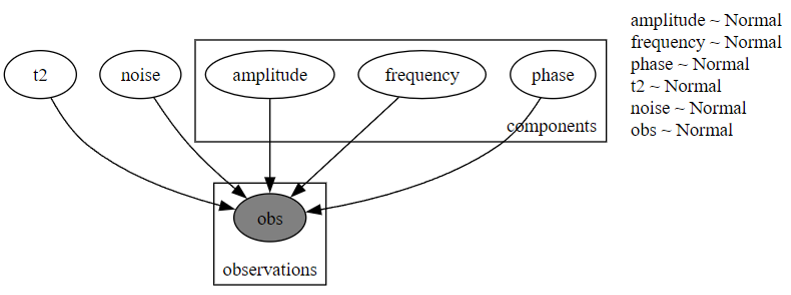
I have been working on a dummy experiment with potential ramifications for optimised NV Ramsey magnetometry in which I randomly generate N sine waves with local latent variables of (Amplitude, frequency, phase); I sum these and apply a decaying Gaussian wavepacket after which I add on some Gaussian noise. These introduce global latent variables, T2 and sigma.
In my experience so far, I have ran into numerous consistent issues:
-
Noise is consistently overestimated, even when using priors that constrain it to near-zero, or even tight priors centred at its true value.
-
Amplitude is consistently underestimated. This is sometimes observed with frequency as well.
-
Phases often don’t change their position during inference.
-
When the number of sines assumed to be present in the signal M is larger than N I am not achieving parsimony.
TLDR, my method is clearly quite unstable. Different seeds do produce different minima, which I believe only validates my conclusion. I have tested using perfect priors, and yet I still notice a decay.
So far, I have attempted to use Gaussian priors and posteriors for my local latent variables, and have exhausted the possibilities of using MLE or MAP on the globals. I have now moved onto using inverse-Gamma distributions for T2 and noise, and use a model like so:
    def model(self, t: torch.Tensor, observed_signal: torch.Tensor):
        # Assure that the input signals are consistent with the asserted datatype expected throughout inference.
        t = t.to(dtype=self.dtype, device=self.device)
        observed_signal = observed_signal.to(dtype=self.dtype, device=self.device)

        @poutine.scale(scale=1.0 / len(t))  # To normalise -ELBO.
        def _model():
            with pyro.plate("components", self.M):
                # Sample a value from the prior distributions.
                amplitude = pyro.sample("amplitude", self.amplitude_prior)
                frequency = pyro.sample("frequency", self.frequency_prior)
                phase = pyro.sample("phase", self.phase_prior)


            T2 = pyro.sample("t2", self.t2_prior)
            sigma = pyro.sample("noise", self.noise_prior)


            decay = torch.exp(-(t / T2) ** 2)

            y_pred = decay * torch.sum(
                amplitude.unsqueeze(-1) * torch.sin(frequency.unsqueeze(-1) * t + phase.unsqueeze(-1)), dim=0)

            with pyro.plate("observations", len(t)):
                pyro.sample("obs", dist.Normal(y_pred, torch.abs(sigma)), obs=observed_signal)

        return _model()
For reference, the priors are generated during Class initialisation are done like so:
        # Setup priors. All local latent params are assumed to be distributed according to a Normal dist.
        self.amplitude_prior = Normal(self.prior["Amplitude"][0], self.prior["Amplitude"][1])
        self.frequency_prior = Normal(self.prior["Frequency"][0], self.prior["Frequency"][1])
        self.phase_prior = Normal(self.prior["Phase"][0], self.prior["Phase"][1])

        # Priors for Global Latent Variables, assuming they're present in the signal.
        if self.decaying:
            self.t2_prior = InverseGamma(self.prior["T2"][0], self.prior["T2"][1])
        if self.noisy:
            self.noise_prior = InverseGamma(self.prior["Noise"][0], self.prior["Noise"][1])
Seeing as that I consistently underestimate, I have a suspicion that my instability is caused by inherent bimodality across these parameters. If you look at the equation that I am using in my model:
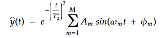
you can see that there is room for much degeneracy. For example, you can obtain the same output by flipping the sine of the amplitude, and adding pi to the phase; or similarly you can flip the sign of the frequency and modify the phase to be (pi - estimated value)…
I have tracked the evolution of these parameters during operation, and have found that some oscillate around that true value, but more often than not steadily decrease. My thoughts were that the bimodality of these local parameters was preventing learning, and I assume that I need to apply some kind of probability distribution transformation to enforce unimodality, since I can’t simply enforce a positivity constraint without preventing parsimony in cases where M>N.
It’s all becoming quite a lot to keep track of. I’ve been using Adam as my optimiser, experimenting with gradient clipping thresholds, learning rates (and their decays), momenta and L1 regularisation but ultimately these have been more of a hail Mary in terms of finding something that is stable across a range of signals. If you have gotten this far, I could use some help in figuring out if I should be using probability transforms, and if so, what would be applicable to my problem. I still have to juggle the boundaries of my phase on top of all this…
Thank you for reading this. If you feel like you need more information from me, please do let me know. This is my first time making a forum post anywhere, I believe I have been sufficiently frustrated by this problem to embrace the support of similarly caffeinated strangers…