Hello everyone,
Here is an bird’s eye view of what I am trying to do with my specific question coming in the second paragraph below. I am simulating a dynamical system using differential (or difference equations) with the goal of estimating the parameters of the equations. In reality, we don’t know the exact value of these parameters and we treat them as random variables. My goal is to derive a posterior distribution for these parameters given their prior distribution and a set of measurements. As a starting point I am working with the following system which uses the difference and measurement equations below
where the parameter a \sim \mathcal{N} (\mu, \sigma_a^2) is normally distributed and is the parameter we care to estimate. x_t is the unknown state at time t, y_t is the measurement at time t, and \nu \sim \mathcal{N} (0, \sigma^2) is the measurement noise, which is zero mean normally distributed noise with variance \sigma^2. I have created the Jupyter notebook markov_model.ipynb and the utilities.py with all the helper functions. Both can be found at my GitHub repo. The pipeline is the following:
- Generate data with the true generating process, and
- Use stochastic variational inference to estimate the posterior of the parameter.
For the guide function, I am using AutoNormal and for the loss function I am using TraceELBO. Even though the specific example is linear and as far as I understand there are already implementations in Pyro that deal with linear models with Gaussian noise, my goal is to work with nonlinear dynamical systems with non-Gaussian distributions. Also, I think it is important for any researcher to have some understanding of what is happening under the hood of all the software machinery they are using.
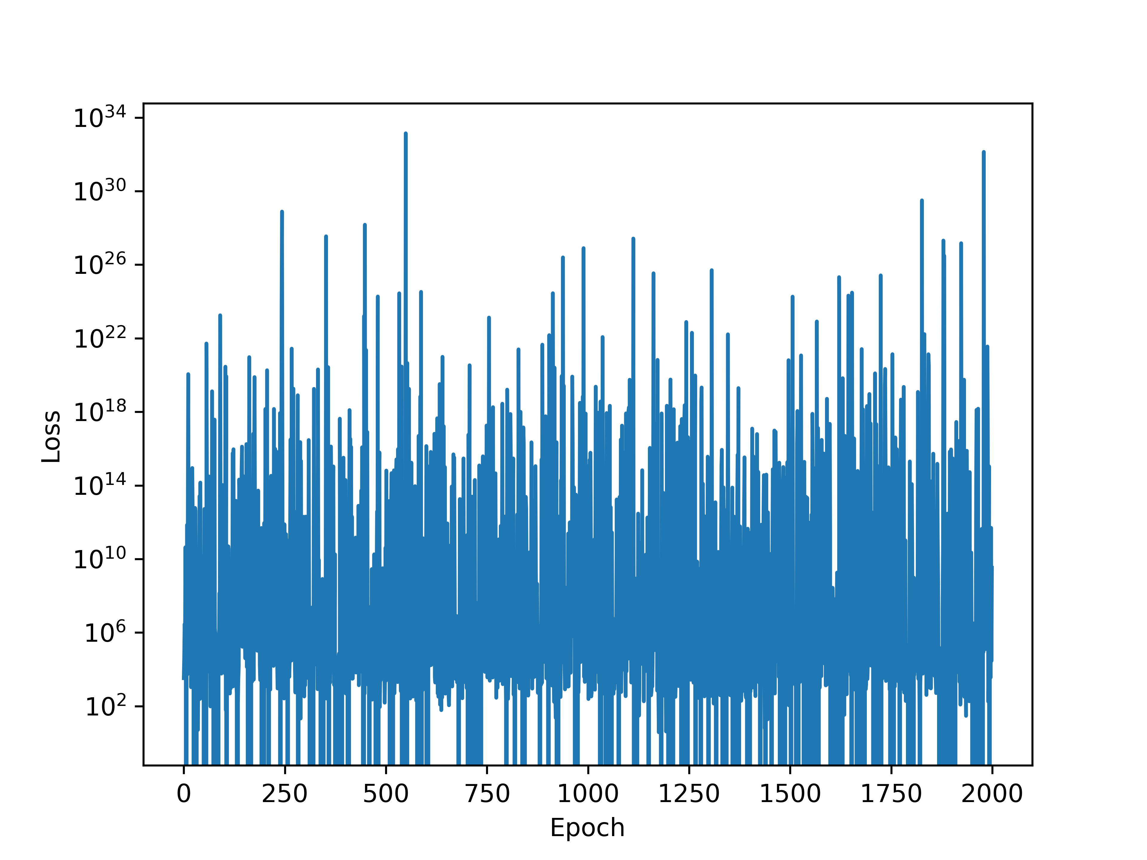
The problem is the following: the loss function does not decrease as a function of the training epoch and its really noisy as can be seen in the image below. Most importantly, the posterior has pretty much the same mean as the prior and I have a feeling if I let the script run for more epochs it will end up having the same variance as well. This prevents me from making any meaningful statements about the parameter involved in the difference equation above. Could someone look at my code and see where I might have gone wrong? Any help to resolve this issue will be highly appreciated.