First of all, thank you for the amazing package!
I’ve been using the Ordinal Regression example, but I’d like to enhance with a more principled prior as suggested by M.Betancourt in Case Study on Ordinal regression (section 2.2).
However, I’m struggling to create cut point “parameters” that would be optimized by the MCMC alongside the other random variables. It might be an improper usage of the numpyro.param() statement and/or numpyro.factor()
The expected behaviour would be that cutpoints will change during the MCMC run, however, they stay equal to their initial values.
Helper function for the lpd of the prior model as per Michael’s blog:
def induced_dirichlet_lpdf(c,alpha,phi):
‘’’
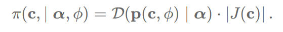
Function to calculate the log-density for induced Dirichlet prior
Based on: Ordinal Regression
INPUTS:
- c:jnp.array: cut point array (length=number of categories less 1)
- alpha:jnp.array: concentration for Dirichlet distribution
- phi:float: anchor point honouring M. Betancourt’s implenentation
RETURNS:
- p:jnp.array: vector of implied probabilities for each category
- lpd:float: log-density for the prior (include log det Jacobian )
'''

K=len(c)+1 # number of categories
p=jnp.zeros((K,),dtype=float) # proba
J=jnp.zeros((K,K),dtype=float) # Jacobian

sigma=expit(phi-c) #Logistic function // CDF

# Induced Ordinal Proba
p=p.at[0].set(sigma[0])
p=p.at[1:-1].set(sigma[:-1]-sigma[1:])
p=p.at[-1].set(sigma[-1])

# Baseline column of Jacobian
J=J.at[:,0].set(1.0)

# Diagonal entries of Jacobian
rho=jnp.multiply(sigma,1-sigma) # partial deriv.
i,j=jnp.diag_indices(K-1) # needs to start from index 1:
# diagonal elements
J=J.at[..., i+1, j+1].set(-rho)
# off-diagonal elements
J=J.at[..., i+1, j+1].set(rho)

_,log_det=jnp.linalg.slogdet(J)

lpd=dist.Dirichlet(alpha).log_prob(p)+log_det

return p,lpd
and the model to run it:
def model(covariates,obs=None):
‘’’
Simple Ordinal regression with Dirichlet induced prior for the latent cut points
‘’’
num_classes=3 #fixed for now
dim_cov = covariates.shape[1]
N=covariates.shape[0]

cutoff_init=jnp.linspace(-2,2,num_classes-1)
anchor_point=0.0
concentration_prior=jnp.array([1,1,1])

beta=numpyro.sample('beta',dist.Normal(0,10).expand([dim_cov]).to_event(1))
mean_pred = jnp.dot(beta,covariates.T)

# parameters for cut points
c_y=numpyro.param('c_y',init_value=cutoff_init,constraint=dist.constraints.ordered_vector)

# get their log-density
p_y,log_density=induced_dirichlet_lpdf(c_y,concentration_prior,anchor_point)

# add to the overall log likelihood
numpyro.factor("induced_prior_transformation", log_density)

if obs is None:
    numpyro.deterministic('mean_pred',mean_pred)
    numpyro.deterministic('c_y',c_y)
    numpyro.deterministic('p_y',p_y)

with numpyro.plate("N", N) as idx:
    return numpyro.sample("obs", dist.OrderedLogistic(mean_pred,c_y), obs=obs)
I’ve searched for any similar threads, but the only helpful one was Implicit priors, but it wasn’t very clear around param() vs factor().
Any help would be greatly appreciated! I’m happy to contribute it to the example if it’s useful.