Hi everyone,
I’ve been trying to implement high dimensional ODE models in numpyro using NUTS and this forum has been a great help thusfar! I was able to speed up my code immensely. Using a jax implementation I can now obtain maximum likelihood estimates of my full model in a few minutes.
These estimates are helpful (for instance, I’ve learned that many of the parameters are highly correlated) but I would like to utilize prior information and obtain a posterior distribution over the parameters.
Hence, I want to do a ‘fully Bayesian’ analysis with MCMC. Unfortunately this has been giving me lots of trouble. For starters, my full model (with about 60-70 parameters, excluding likelihood sigma’s) with real data simply does not converge. It takes an immense amount of time and then after a day or so the kernel simply breaks down and resets.
Therefore, I’ve been trying to work with synthetic/fake data and a smaller model. However, even very small models have been challenging and I have yet to efficiently run an ODE model and obtain reasonable rhat statistic and effective sample size, or even properly find the parameters that generated the data back. I’ve also noticed that generally some chains take much longer than others, which suggests that some initializations are more problematic than others. I’ve also tried using stricter priors to little avail. I’ve not yet experimented with different likelihood functions because right now i’m not even adding noise to the fake data.
I’ve created the simplest ODE system I could think of: system of two first order linear ODEs with each one parameter, and a dataset of 3 fake individuals and with 12 timesteps each.
I’ve put the model in this editable colab notebook: Google Colab
Running the model for 4 NUTS chains 1000 warmup + 1000 samples takes >30 minutes with default settings. And still the diagnostics are extremely bad (n_eff = 2, rhat is almost 40) and the parameters are not properly identified, even though a traditional minimizer finds the correct MLE is splitseconds.
Can someone please help me understand why the model performs the way it does? I would love to use numpyro to run the more complex ODE models but right now that seems impossible.
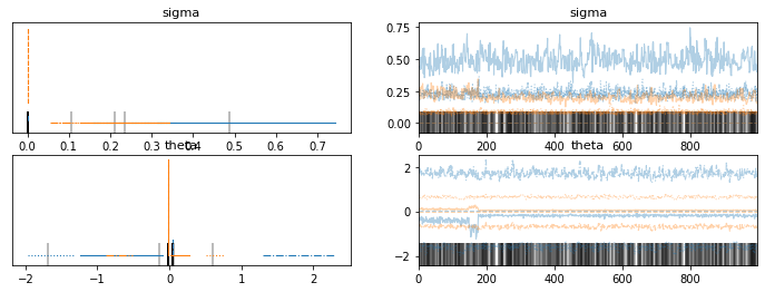
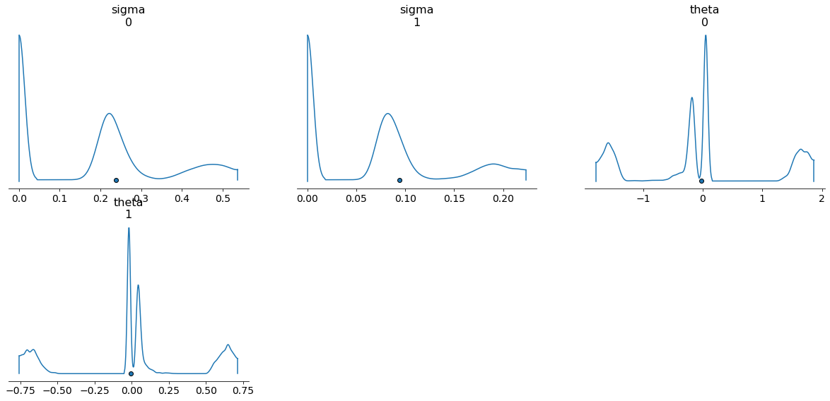
@martinjankowiak thanks a lot! enable_x64 does speed up NUTS immensely. It went from 35 minutes to 2 minutes. However, I did not get reasonable results for 1000 warmup + 1000 samples and 4 chains with rhat of 10 for the thetas, rhat of 4 for the sigmas, n_eff of about 2, and 511 divergences. Furthermore I got much more uncertainty (with incorrect point estimates) than expected based on the minimization results.
I’ve attached the density plots, which look really strange, and the trace plots also suggest very poor mixing:
Thanks for thinking along! Sorry I didn’t notice you edited the colab notebook. The result seemed somewhat reasonable when you used 500 samples and 1 chain but when I put 1000 samples and 4 chains, I find the same issues in the notebook (Google Colab).
Btw, if I further lower atol/rtol to 1.4e-8 and maxsteps=1000 I also get poor results.
Any other suggestions?
@martinjankowiak, I ran NUTS for 10,000 samples and a single chain and now get perfect results (although it did take almost 30 minutes for this tiny model). Any idea why the multiple chains are not mixing?
I would think that init_to_sample() should work well, as it simply samples the initial parameters from the normal(0,1) prior. I don’t understand why the sampler would be sensitive to initial conditions in this case.
I’m a bit confused about what you mean by a plot of the joint log density, do you mean a pair plot of the parameters? I’ve added it to the Google Colab
It looks good for the single chain (with some expected correlation between the parameters) but very peculiar when I run multiple chains.
Also when running multiple chains 2000 samples it’s again apparent that some chains take (much) longer than others (shortest took 50 seconds, longest took 15 minutes). Why did you actually run it for just a single chain? My understanding is that one should use at least three-four chains and that these should mix well in order to validate the identified posterior?
Btw, i also checked if the chain method matters but it doesn’t (sequential also gives poor mixing).
your model defines a log joint density. it is a scalar function of the continuous random variables. it can be plotted (or slices of it can be plotted depending on the dimensionality) without using any numpyro inference machinery. in particular without drawing any samples.
i haven’t looked at your ode in detail. are you sure it’s actually a well posed problem? e.g. is it approximately unimodal? will the ode integrator tend to blow up for large |theta| etc?
i don’t know why it’s slow with multiple chains. maybe it’s colab. maybe it’s that odeint doesn’t like being run like that. i imagine it’s more of a jax issue than a numpyro issue…
if you have good reason to believe that a model is approximately unimodal there’s arguably no reason to run multiple chains. sure, multiple chains are useful for diagnostics and are probably good practice when you can afford the extra compute. but a single chain that is sufficiently long can also be used to compute r_hats etc.
Just an input that you might try different random seeds on single chain, or exploring each chain in your multi-chain run, to see the issue. It seems to me that this is not a problem of multiple chains. Poor mixing seems to indicate that there is a problem with the model.
@martinjankowiak
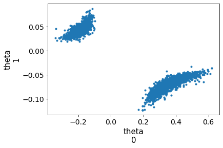
At the moment the only ‘issue’ that I can think of with this simple and also more complex ODE models is the high correlation between parameters. In this case the correlation is very very high, and when I run two chains I get the pair plot below. That suggests to me that the posterior is multimodal (so not unimodal) and that the different chains get stuck around different modes. Does that seem plausible?
I’m just not sure how to combat this, two options that I’m thinking about:
More stringent priors, but these will be difficult to set with real world data.
To first run optimization and fix some of the parameters that are very highly correlated (I can check if the log posterior is sensitive to them using sensitivity analysis for instance)
But both of these are suboptimal. I had hoped that NUTS would work well regardless of correlations between parameters.
strong correlation between parameters isn’t necessarily a huge problem unless the number of dimensions is very high in which case it might be.
widely separated modes can be a big problem. i have no idea what class of ODEs you’re interested in but anything you can do to make the model more identifiable, whether that means more stringent priors, fixing certain parameters, breaking symmetries through reparameterization, etc, may help a lot
I’m interested, for now, in (simple but) large linear ODE systems with many parameters (up to 70-80). So (much) larger versions of the simple model in the colab notebook. Hence, it worries me that identifiability issues already appear to play a role even for this small model.
Unfortunately also with enable_x64 the larger model takes much too long to run.
Nevertheless, I am able to find decent results with minimization methods. So I’m thinking I’ll focus on variational inference for now. I have a few questions about that.
Firstly, does it make sense to implement this in numpyro (which i’m now comfortable with), or should I use pyro instead, which I haven’t used before?
Secondly, I’ve changed the colab example (Google Colab) to using AutoDelta and AutoLaplaceApproximation.
However, for some reason with AutoDelta (and minimize with BFGS, or ADAM) i’m finding an optimum with extremely high error. Is my implementation off somehow?
I generally get reasonable (frequentist) estimates with nonlinear least squares and then the covariance approximation with the Hessian. But I would like estimates that include sigma’s for the measurement model and be able to express different prior distributions. So to that end I want to use (num)pyro.
Finally, based on a previous topic @fehiepsi updated AutoLaplaceApproximation to include the hessian_fn option to avoid forward autodiff errors regarding custom vjp functions when using odeint. I can see it on Github. Yet somehow this option is not yet working in the latest pip installed numpyro version? Or am I missing something?
Thanks! I got it to work by installing from source :). Any suggestions why the AutoDelta and AutoLaplaceApproximation are finding such poor results while nonlinear least squares does work? Maybe I’m misunderstanding how to create such a model (Google Colab)
This is how I’m calling the model, and it’s giving me results with extremely high error: (it doesn’t matter whether I use BFGS or Adam, or AutoDelta or AutoLaplaceApproximation)
priors are different: you might try to use a prior like Normal(0, 100) or even ImproperUniform
sigma is latent: you might try to fix it to some value
the params are not optimized yet: you might try l-bfgs-experimental-do-not-rely-on-this method for Minimizer or setting smaller learning rate, much longer svi iterations for Adam,…