Hey @fehiepsi, thank you for your reply!
Regarding the priors, the issue I see with that is that the variances of these errors terms are fixed and known when we do inference. So I’m not sure putting a prior on them will help.
Also, the following script will do as you ask (though this is for Stochastic VI only, to keep it simple). It’ll save 4 images to the directory in which you run it. One named “losses” and 3 others named "Posterior for ".
import numpy as np
import pandas as pd
from datetime import date
import matplotlib.pyplot as plt
import pyro
from pyro.optim import SGD, Adam
from pyro.infer import SVI, Trace_ELBO
# from pyro.infer.mcmc import NUTS, MCMC
import pyro.distributions as dist
from pyro.contrib.autoguide import AutoLowRankMultivariateNormal, AutoDiagonalNormal, AutoGuide, AutoDelta
import torch
from torch.distributions import constraints
pyro.enable_validation(True)
pyro.set_rng_seed(42)
# Define some plotting functions
def get_df_samples(guide, var_name, num_samples = 500):
"""
This returns a dataframe with samples of all variables starting with the string 'var_name'. In other words,
this gives us a way to gather posterior samples of certain latent variables through time. The output
has samples down the columns and time-indexed latent variables across the columns.
"""
samples = []
for i in range(num_samples):
post_sample = guide()
if i == 0:
names = [nm for nm in post_sample if nm.startswith(var_name)]
names = sorted(names, key = lambda x: int(x.split('_')[-1]))
sample = {nm: post_sample[nm].item() for nm in names}
samples.append(sample)
return pd.DataFrame(samples)[names]
def standard_plot(figsize=(12,5)):
fig, ax = plt.subplots(figsize=figsize)
ax.grid(True)
return fig, ax
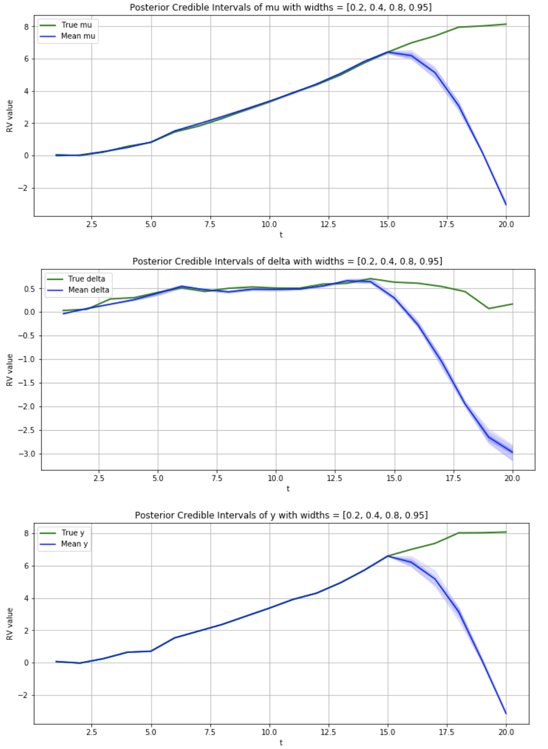
def plot_true_vs_post_samples(samples, var_name, true_vars,
credible_interval_widths = [.2, .4, .8, .95],
figsize=(12,5)):
"""
This creates a time series plot showing true latent variable values overlaid with posterior
credibly intervals.
"""
# Calculate data for the plot
percentiles = sorted([.5+sn*w/2 for w in credible_interval_widths for sn in [1,-1]])
samp_percentiles = samples.quantile(percentiles)
mean_sample = samples.mean()
fig, ax = standard_plot(figsize)
# Plot true values first
true_var_nms = list(ky for ky in true_vars if ky.startswith(var_name))
true_var_nms = sorted(true_var_nms, key = lambda x: int(x.split('_')[-1]))
var_true_by_t = pd.Series({t+1: true_vars[true_var_nms[t]].item() for t in range(len(true_var_nms))})
t_index = var_true_by_t.index
ax.plot(t_index, var_true_by_t.values, label = 'True ' + var_name,
color='green', linewidth=2)
samp_t_index = [int(nm.split('_')[-1]) for nm in samp_percentiles]
# Plot mean sample values
ax.plot(samp_t_index,
mean_sample.values, label = 'Mean ' + var_name, color='blue')
# Plot posterior credible intervals
for w in credible_interval_widths:
above = samp_percentiles.loc[.5 + w/2, :]
below = samp_percentiles.loc[.5 - w/2, :]
ax.fill_between(samp_t_index, above, below, alpha=.1, color='blue')
ax.legend()
ax.set(xlabel='t',
ylabel='RV value',
title = f'Posterior Credible Intervals of {var_name} with widths = {credible_interval_widths}')
return fig, ax
# Generate fake data according to a local linear trend model and perform inference to recover the true synthetic values.
if __name__ == '__main__':
# Some true synthetic data generation parameters
T = 20 # Number of time indices for which we generate data
tau = 15 # The last time index for which we observe y
ep_scale = 1 # Standard deviation on epsilon error
eta_scale = 1 # Standard deviation on eta error
xi_scale = 1 # Standard deviation on xi error
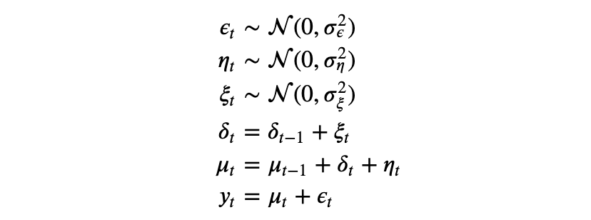
# Our model, a stochastic function. This is our data generation process according to a local linear trend model.
def model():
delta_s, mu_s, y_s = {'delta_0': 0}, {'mu_0': 0}, {'y_0': 0}
for t in range(1, T+1):
# Variable names
delta_nm = 'delta_{}'.format(t)
delta_nm_prev = 'delta_{}'.format(t-1)
mu_nm = 'mu_{}'.format(t)
mu_nm_prev = 'mu_{}'.format(t-1)
y_nm = 'y_{}'.format(t)
# Pyro random variables
delta_s[delta_nm] = pyro.sample(delta_nm, dist.Normal(delta_s[delta_nm_prev], ep_scale))
mu_s[mu_nm] = pyro.sample(mu_nm, dist.Normal(mu_s[mu_nm_prev] + delta_s[delta_nm], eta_scale))
y_s[y_nm] = pyro.sample(y_nm, dist.Normal(mu_s[mu_nm], xi_scale))
del delta_s['delta_0'], mu_s['mu_0'], y_s['y_0']
return delta_s, mu_s, y_s
# Generate synthetic data
delta_s_true, mu_s_true, y_s_true = model()
all_true_vars = {**delta_s_true, **mu_s_true, **y_s_true}
# Condition on those observations
observations = {'y_{}'.format(t):y_s_true['y_{}'.format(t)] for t in range(1, tau+1)}
conditioned_model = pyro.condition(model, data=observations)
# Create a simple guide
guide = AutoLowRankMultivariateNormal(conditioned_model, 10)
# Perform Inference (using VI) and plotting the VI loss.
pyro.clear_param_store()
svi = SVI(conditioned_model, guide, Adam({"lr": 0.1}), Trace_ELBO())
losses = []
num_steps = 1200
for t in range(num_steps):
losses.append(svi.step())
if not (t % 100):
print(losses[-1])
fig, ax = standard_plot()
ax.plot(range(len(losses)), losses)
_ = ax.set(xlabel='iterations', ylabel='ELBO Loss', title = 'Loss by VI iterations')
fig.savefig('losses.png')
# Inspect posterior samples
credible_interval_widths = [.2, .4, .8, .95]
num_samples = 500
for var_name in ['mu', 'delta', 'y']:
samples = get_df_samples(guide, var_name, num_samples)
fig, ax = plot_true_vs_post_samples(samples, var_name, all_true_vars, credible_interval_widths)
fig.savefig(f'Posterior for {var_name}.png')