Model of time series with different lengths

I am working on a model of time series where each time series may be of different length. For concreteness, I am modeling the outputs of different instruments over time where each of the instruments is brought online at a different time. A simplified version of the model is

\begin{aligned} \mathbf{z}_{i}&\sim\mathsf{RandomWalk}\left(\tau_i\right)\\ y_{it}&\sim\mathsf{Normal}\left(z_{it},\sigma_i\right) \end{aligned},

where \mathbf{z}_i\in\mathbb{R}^T is the latent time series for the i^\text{th} instrument, T is the length of the observation period, \tau_i is the scale of the random walk innovations of the i^\text{th} instrument, y_{it} is the observation for the i^\text{th} instrument at time t, and \sigma_i is the scale of the observation noise for the i^\text{th} instrument.

Say the first instrument is brought online at the beginning of the observation period, then I want to introduce T parameters for \mathbf{z}_1. If the second instrument is brought online half-way through the observation period, I want T/2 parameters for \mathbf{z}_2. Such a jagged structure is of course difficult in numpyro.

What I’ve considered so far

One approach is to forget about the problem and parameterize \mathbf{z} with a dense parameter matrix. But that means I use about twice the number of parameters I actually need.

Another approach is to sample the time series for each instrument independently in a for loop. But I have about 1,000 instruments, and unrolling the loop in jax.jit seems problematic.

I could sample one big vector \xi of length m=\sum_{i=1}^n T_i, where n is the number of instruments and T_i is the number of observations I have for instrument i. Then construct indices to scatter \xi into the dense matrix z. That seems fiddly for two reasons: first, constructing the indices; second, placing an appropriate prior on \xi such that z has the desired distribution.

Ideas on how to best parameterize the model would be great; thanks for your time!
depends on details but often the best way to deal with something like this is do everything in a vectorized fashion using z_T of length T_max for all time series and then using mask to mask out missing observations and the like.

do you expect to use svi?

1 Like

Thanks for the note! The approach I’m currently using is to have a dense matrix of z and then index for observations. The model looks as follows.

def model(i: jnp.ndarray, t: jnp.ndarray, y: jnp.ndarray):
    """
    Args:
        i: Integer array of length `m` with values in `[0, n)`, 
            where `m` is the total number of observations and `n` 
            is the number of instruments.
        t: Integer array of length `m` with values in `[0, T]`,
            where `T` is the length of the observation period.
        y: Float array of length `m` corresponding to observation
            of instrument `i` at time `t`.
    """
    # Sample tau and sigma scales, both of length `n`.
    ...

    with numpyro.plate("z-plate", n):
        # Float array of shape `(n, T)`.
        z = numpyro.sample("z", RandomWalkDistribution(taus))

    with numpyro.plate("y-plate", m):
        y_hat = z[i, t]
        numpyro.sample("y", Normal(y_hat, sigmas[i], obs=y)

I think it’s not quite what you had in mind with masking but maybe similar in spirit?

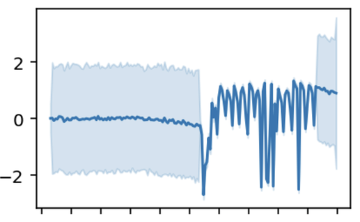
Here is an example of the inferred time series. The large variance in the beginning is due to the instrument only coming online about half way through the observation period. The large variance at the end are out-of-sample predictions.

This probably hasn’t quite converged, because I’d expect to see a square-root “cone” for the prediction uncertainty due to the random walk. Ideally, I’d like to remove the parameters in the first half because I know they’re going to converge to the prior and are not interesting.

Yes, I’m using SVI for the inference. The full model has about 350k parameters so sampling seemed maybe a bit ambitious.

As an aside, a random walk is of course not a great model given the periodicity of this particular example, but it’s a starting point.

you presumably need to mask out fake observations in numpyro.sample("y", Normal(y_hat, sigmas[i], obs=y)

Sorry, I should’ve made things clearer. y is a vector of all the observed values. Suppose I have a dense matrix Y of observations with shape (n, T), some of which are missing. Then y is defined as follows.

from jax import numpy as jnp

i, j = jnp.where(~jnp.isnan(Y))
y = Y[i, j]
# y is a vector of length (~jnp.isnan(Y)).sum().

Given this setup, I think I don’t need to mask the observations because y has already been restricted to the available data without missing values. I may of course have misunderstood.

In practice, I never construct the dense Y because it would consume too much memory.

i think it’s probably harder to do better than you’re doing and a factor of 2 isn’t a huge cost. are you using a gpu? gpus like vectorized tensor ops

Great, thank you for the additional information. In practice, I’m looking at about a factor of five in terms of dense vs observed data (turns out I got my numbers wrong initially). But maybe that bottleneck can be overcome more easily by adding a GPU to my VM instead of changing the implementation.

Thanks for the fast replies.

to limit memory/time per step it’s probably easiest to introduce data subsampling so that you only consider a fraction of time series in each optimization step

1 Like