Model Based Machine Learning chapter 3, loss oscillating

Hi, I am working on Chapter 3, on the following model:

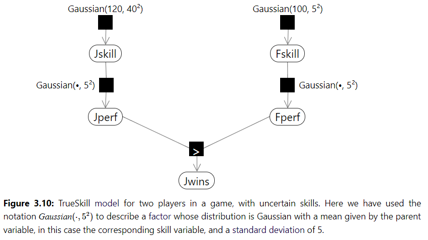
We sample Jill skills from a Gaussian distribution, and we use that sampled value to sample performance form N(Jillskill, 5). We do the same for Fred. We have a deterministic factor checking if Jill wins. We expect that if Fred wins twice, his skill is believed to be higher.

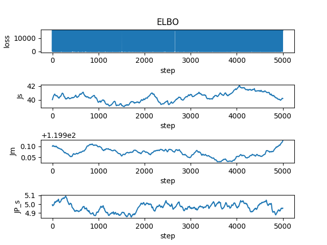
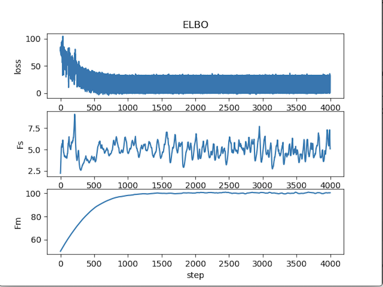
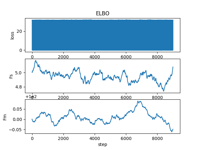
I plot the loss and it is just oscillating, see the plot below. Fm and Fs are the mean and standard deviation of Fred with input [0,0] (Jill lost twice)

Here is the code, can you help me find where is the problem?

import matplotlib.pyplot as plt
import numpy as np
import torch
import pyro
import pyro.distributions as dist
import pyro.infer
import pyro.optim
from pyro.optim import Adam
import torch.distributions.constraints as constraints
def scale(Data):
    Jskill = pyro.sample('JS', dist.Normal(120.,40.))
    Jperf = pyro.sample('JP', dist.Normal(Jskill, 5.))
    Fskill = pyro.sample('FS', dist.Normal(100.,5.))
    Fperf = pyro.sample('FP', dist.Normal(Fskill, 5.))
    Jwin = torch.tensor([0.0])
    if Fperf<Jperf:
        Jwin = torch.tensor([1.0])
    with pyro.plate("plate", len(Data)):
        a= pyro.sample('JW', dist.Bernoulli(Jwin), obs=Data)

def guide(Data):
    J_m = pyro.param('J_m', torch.tensor(120.0))
    J_s = pyro.param('J_s', torch.tensor(40.0), constraint = constraints.positive)
    F_m = pyro.param('F_m', torch.tensor(100.0))
    F_s = pyro.param('F_s', torch.tensor(5.0), constraint=constraints.positive)
    Jp_s = pyro.param('JP_s', torch.tensor(5.0), constraint=constraints.positive)
    Fp_s = pyro.param('FP_s', torch.tensor(5.0),constraint=constraints.positive)
    Jskill = pyro.sample('JS', dist.Normal(J_m,J_s))
    Jperf = pyro.sample('JP', dist.Normal(Jskill, Jp_s))
    Fskill = pyro.sample('FS', dist.Normal(F_m,F_s))
    Fperf = pyro.sample('FP', dist.Normal(Fskill,Fp_s))


Data =  torch.tensor([0.0, 0.0]) # Jill loses twice

pyro.clear_param_store()
adam_params = {"lr": 0.001, "betas": (.9, .999)}
optimizer = Adam(adam_params)
svi = pyro.infer.SVI(model=scale,
                     guide=guide,
                     optim=optimizer,
                     loss=pyro.infer.Trace_ELBO())


losses, a,b  = [], [], []
num_steps = 9000
for t in range(num_steps):
    losses.append(svi.step(Data))
    a.append(pyro.param("F_s").item())
    b.append(pyro.param("F_m").item())

plt.subplot(3,1,1)
plt.plot(losses)
plt.title("ELBO")
plt.xlabel("step")
plt.ylabel("loss");

plt.subplot(3,1,2)
plt.plot(a)
plt.xlabel('step')
plt.ylabel('Fs')

plt.subplot(3,1,3)
plt.plot(b)
plt.xlabel('step')
plt.ylabel('Fm')
plt.savefig('Floss.png')
print('FS = ',pyro.param("F_s").item())
print('FP = ', pyro.param("F_m").item())

I decided to simplify the model, now Jill is playing with a machine with constant skill=150 and performance = 150.

Also I put 1000 data points (this modified linearly the loss range) where Jill always wins, so I assumed the estimation of Jill performance is supposed to get better.

The code below returned J_StandarDeviation = 40.2089729309082
J_mean = 120.02542877197266
JPerformanceStandarDeviation = 4.954901218414307


Lets assume Jill plays with a robot that always has skill 150

import matplotlib.pyplot as plt
import numpy as np
import torch
import pyro
import pyro.distributions as dist
import pyro.infer
import pyro.optim
from pyro.optim import Adam
import torch.distributions.constraints as constraints

def scale(Data):
    Jskill = pyro.sample('JS', dist.Normal(120.,40.))
    Jperf = pyro.sample('JP', dist.Normal(Jskill, 5.))
    Jwin = torch.tensor([0.0])
    if 150<Jperf:
        Jwin = torch.tensor([1.0])
    with pyro.plate("plate", len(Data)):
        a= pyro.sample('JW', dist.Bernoulli(Jwin), obs=Data)

def guide(Data):
    J_m = pyro.param('J_m', torch.tensor(120.0))
    J_s = pyro.param('J_s', torch.tensor(40.0), constraint = constraints.positive)
    Jp_s = pyro.param('JP_s', torch.tensor(5.0), constraint=constraints.positive)
    Jskill = pyro.sample('JS', dist.Normal(J_m,J_s))
    Jperf = pyro.sample('JP', dist.Normal(Jskill, Jp_s))


Data =  torch.tensor([1.0]*1000) # Jill wins 1000 times

pyro.clear_param_store()
adam_params = {"lr": 0.001, "betas": (.9, .999)}
optimizer = Adam(adam_params)
svi = pyro.infer.SVI(model=scale,
                     guide=guide,
                     optim=optimizer,
                     loss=pyro.infer.Trace_ELBO())

losses, a,b  = [], [], []
num_steps = 5000
for t in range(num_steps):
    losses.append(svi.step(Data))
    a.append(pyro.param("J_s").item())
    b.append(pyro.param("J_m").item())

plt.subplot(5,1,1)
plt.plot(losses)
plt.title("ELBO")
plt.xlabel("step")
plt.ylabel("loss");

plt.subplot(5,1,3)
plt.plot(a)
plt.xlabel('step')
plt.ylabel('Js')

plt.subplot(5,1,5)
plt.plot(b)
plt.xlabel('step')
plt.ylabel('Jm')
plt.savefig('Tuesday.png')
print('JS = ',pyro.param("J_s").item())
print('JP = ', pyro.param("J_m").item())

Note that the loss range has increased considerably, in fact it scales linearly with respect to the Data size.

I also changed the standard deviation but the results are similar (Js=5,J_s= 120.00334167480469, J_m = 4.953949451446533,JP_s = 5.033321857452393)

It is not clear that SVI is the appropriate approach. The oscillations are due to the fact that the method is stochastic. With much more data and large batches, the oscillations would probably decrease. At the moment, your SVI oscillates between two values, which is strange (I am running the original problem in your first message). You might try computing the posterior directly (see the tutorial with biased coin). It is also possible that the SVI is not appropriate for this problem.

I made the following change to your code (your first submission) in the guide:

#F_m = pyro.param('F_m', torch.tensor(100.0))
#F_s = pyro.param('F_s', torch.tensor(5.0), constraint=constraints.positive)
F_m = pyro.param('F_m', torch.tensor(50.0))
F_s = pyro.param('F_s', torch.tensor(2.0), constraint=constraints.positive)

and I set the lr to 0.1 (instead of 0.001). Rest of the code stays the same. Leaving lr=0.001 would have required 100 times more epochs to see the decrease of the ELBO. The problem you had is that the parameters chosen in the guide were essentially the correct solution. I simply changed two parameters to make sure the solution was away from the expected solution.

I would still experiment with the posterior calculation and marginalization (without the SVI model), which should produce an exact result given sufficient number of samples.

Curious if you’ve made any progress on this with SVI. I have had some success with this problem using MCMC, but I am running into the same problem with SVI. The loss does look better if I set the initial parameter further from the correct answer, but parameter just seems to be working towards the prior specified in the model and is not affected by changing who wins the game. If SVI is not appropriate for the problem, it would be very helpful to gain intuition as to why- perhaps the deterministic node causes a problem with the optimizer?