I’m pretty new to PPLs and have been exploring using Monte Carlo methods to fit some experimental physical data. The problem is the code in numpyro is super slow. I’m using a GPU from colab and it seems to spend abound 5 mins in background_compile() and _execute_compiled() before showing the progress bar. At this point it predicts it will take ~100 hours to complete the sampling for 1000 burn-in, 10000 steps and 250 vectorised chains. This seems quite long to me and I’m wondering if anyone with more experience of this believes this is typical or if my code is not optimal? In addition, the GPU memory pretty instantly reaches 13 GB of the 15 GB once running.
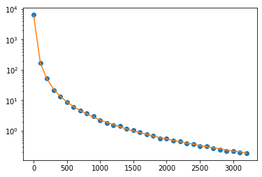
The code is below and hopefully well commented. To test everything I’ve simulated data from the model and have fixed all but one of the variables. The time scale is (0, 3200) ns with $\Delta$t = 100 ns. I have tried solving the ODEs with jax.experimental.ode.odeint but have the same problems.
Thanks in advance for any suggestions/insights. ![]()
![]()
#Import required packages
import jax
import jax.numpy as jnp
from jax.random import PRNGKey
from jax.experimental.ode import odeint

import numpyro
import numpyro.distributions as dist
from numpyro.infer import MCMC, NUTS

import diffrax
import equinox as eqx

#Set all floats to 64 bit
jax.config.update("jax_enable_x64", True)

#Rate equations charge carrier dynamics
class BTDP(eqx.Module):
    """

    Rate equations for the BTD model, as per doi.org/10.1039/d0cp04950f p. 28348
    including trapping, depopulation and background doping.

    Model allows for a non-constant density of traps with depopulation from these
    traps to the valence band.

    Returns
    -------
    [f0, f1, f2]: array
        Array of the rate equations. Dynamics for electron, trap and hole
        concentraions.

    """

    kt: float
    kb: float
    kd: float
    NT: float
    p0: float

    def __call__(self, t, y, args):
        B = self.kb * y[0] * (y[2] + self.p0)
        T = self.kt * y[0] * (self.NT- y[1])
        D = self.kd * y[1] * (y[2] + self.p0)
        f0 = -B - T
        f1 = T - D
        f2 = -B - D
        return jnp.stack([f0, f1, f2])

#JIT compiled function to solve the ODE
@jax.jit
def solve_TRPL_BTDP(kt, kb, kd, NT, p0, N0):
    """

    Solve the ODEs for the BTD model.

    Parameters
    ----------
    kt: float
        k_T trapping rate constant (cm^3 ns^-1).

    kb: float
        k_B bimolecular rate constant (cm^3 ns^-1).

    kd: float
        k_D depopulation rate constant (cm^3 ns^-1) (trap to valence band).

    NT: float
        Trap density (cm^-3).

    p0: float
        Doping density (cm^-3).

    N0: float
        Initial electron concentration (cm^-3).

    Returns
    -------
    sol: array
        Solution to the ODEs.

    """

    #Define equations
    btdp = BTDP(kt, kb, kd, NT, p0)
    terms = diffrax.ODETerm(btdp)

    #Start and end times
    t0 = 0.0
    t1 = 3200.0

    #Initial conditions and initial time step
    y0 = jnp.array([N0, 0.0, N0 + p0])
    dt0 = 0.0002

    #Define solver and times to save at
    solver = diffrax.Kvaerno5()
    saveat = diffrax.SaveAt(ts=jnp.arange(33, dtype=jnp.float64)*100)

    #Controller for adaptive time stepping
    stepsize_controller = diffrax.PIDController(rtol=1e-8, atol=1e-8)

    #Solve ODEs
    sol = diffrax.diffeqsolve(
        terms,
        solver,
        t0,
        t1,
        dt0,
        y0,
        saveat=saveat,
        stepsize_controller=stepsize_controller,
    )
    return sol

#JIT compiled function to calculate the TRPL signal
@jax.jit
def TRPL_BTDP(kt, kb, kd, NT, p0, y0, N0):
    """

    Calculate the TRPL signal for the BTD model.

    Parameters
    ----------
    kt: float
        k_T trapping rate constant (cm^3 ns^-1).

    kb: float
        k_B bimolecular rate constant (cm^3 ns^-1).

    kd: float
        k_D depopulation rate constant (cm^3 ns^-1) (trap to valence band).

    NT: float
        Trap density (cm^-3).

    p0: float
        Doping density (cm^-3).

    y0: float
        Initial TRPL counts (counts).

    N0: float
        Initial electron concentration (cm^-3).

    Returns
    -------
    sig: array
        TRPL signal.

    """

    #Solve ODEs
    sol = solve_TRPL_BTDP(kt, kb, kd, NT, p0, N0)

    #Calculate TRPL signal
    sig = jnp.log10(sol.ys[:, 0]) + jnp.log10(sol.ys[:, 2])

    #Normalise signal and correct for the initial TRPL counts
    sig = sig - sig[0] + jnp.log10(y0)

    return sig

#Standardise the data
def _standardise(x):
    """
    Standardise the data to have a mean of 0 and a standard deviation of 1.

    Parameters
    ----------
    x:  numpy.ndarray
        The data to standardise.

    Returns
    -------
    x:  numpy.ndarray
        The standardised data.
    """
    return (x - x.mean()) / x.std()

#JIT compiled function to standardise the data
standardise = jax.jit(_standardise)

#warm up the JIT
standardise(TRPL_BTDP(1e-15, 1e-18, 0, 1e13, 2e13, 6000, 1e15)).block_until_ready()

#Bayesian model
def model(N0, y, y0):
    """

    Bayesian model for the BTDP model.

    Parameters
    ----------
    N0: float
        Initial electron concentration (cm^-3).

    y: array
        log10 of the experimental TRPL signal.

    y0: float
        Initial TRPL counts (counts).

    """

    #Define priors for the rate constants in log space
    theta = numpyro.sample(
        "theta",
        dist.TruncatedNormal(
            low   = jnp.array([-16]),
            high  = jnp.array([-14]),
            loc   = jnp.array([-15]),
            scale = jnp.array([1]),
        ),
    )

    #Calculate the TRPL signal and standardise
    #Testing with fixed parameters for all but kt
    signal = TRPL_BTDP(10**theta[0], 5e-18, 0, 1e13, 2e13, y0, N0)
    signal = standardise(signal)

    #Define the likelihood
    numpyro.sample("y", dist.Normal(signal, .02), obs=y)

#Generate some simulated data to test the fitting
#time points fixed in model for now
N0 = 1e16
y = TRPL_BTDP(2.2e-15, 5e-18, 0, 1e13, 2e13, 6000, N0)

# create a normal distribution object
normal = dist.Normal(0, .02)

# generate random samples from the normal distribution
noise = normal.sample(PRNGKey(84), (33,))

num_warmup, num_samples = 1000, 10000

#Define the MCMC
mcmc = MCMC(
        NUTS(model, dense_mass=True),
        num_warmup=num_warmup,
        num_samples=num_samples,
        num_chains=250,
        chain_method="vectorized",
        progress_bar=True,
    )
#Run the MCMC with the simulated data and noise
mcmc.run(PRNGKey(78), N0 = N0, y = standardise(y+noise), y0 = 10**(y+noise)[0])
mcmc.print_summary()