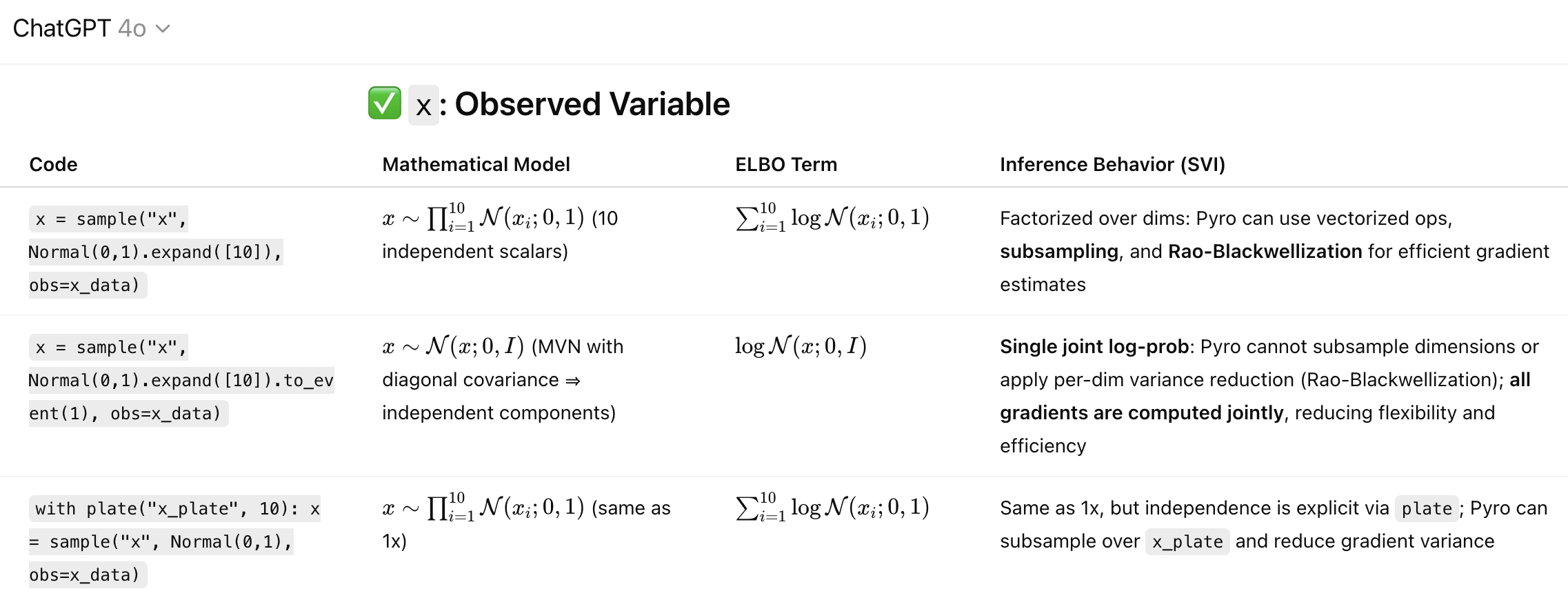
In the model we could have 3 dependency scenarios for observations x:
1x) x = pyro.sample("x", Normal(0, 1).expand([N]))
2x) x = pyro.sample("x", Normal(0, 1).expand([N]).to_event(1))
3x) with pyro.plate("x_plate", N): x = pyro.sample("x", Normal(0, 1))
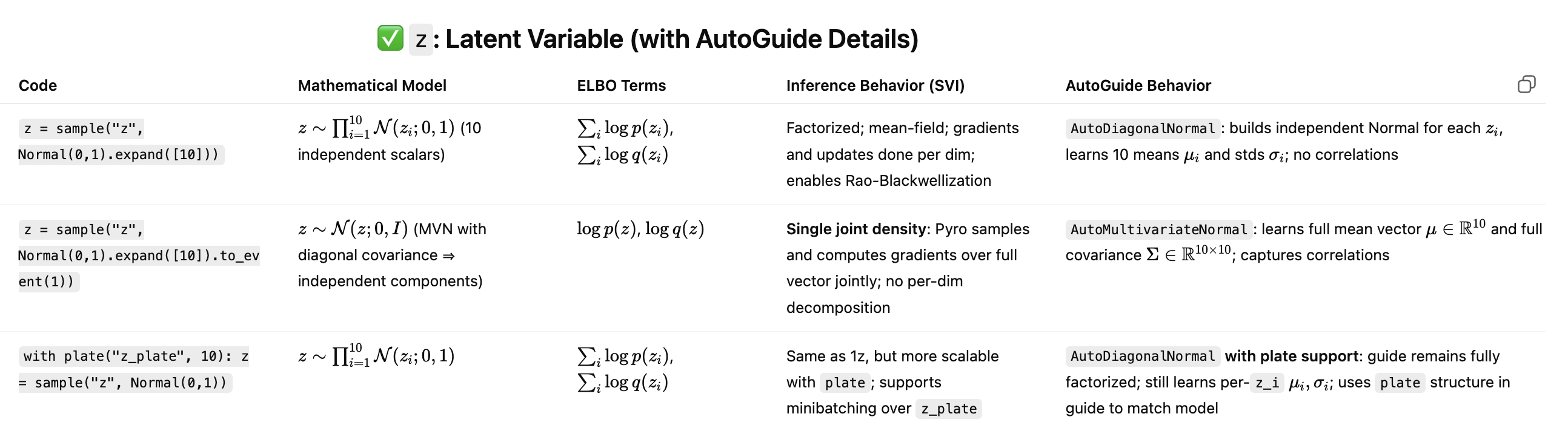
and similarly for latents z:
1z) z = pyro.sample("z", Normal(0, 1).expand([J]))
2z) z = pyro.sample("z", Normal(0, 1).expand([J]).to_event(1))
3z) with pyro.plate("z_plate", J): z = pyro.sample("z", Normal(0, 1))
I want to understand the consequences of each. Below are my questions and guesses, but I’d appreciate someone rewriting the correct consequences for me.
1x) likelihood assumes independence across x ? SVI algorithm cannot exploit this independence for minibatching or fast gradient computations ?
2x) same ?
3x) likelihood assumes independence across x and SVI can exploit for minibatching and gradient computation ?
1z) prior assumes independence across z ? autoguide is AutoMultivariateNormal ? or mean field AutoDiagonalNormal ?
2z) prior assumes independence across z ? autoguide is AutoMultivariateNormal ?
3z) prior assumes independence across z and autoguide is mean field AutoDiagonalNormal ?
if you’re using SVI with reparameterizable latent variables like gaussians, the gradient “follows” the dependency structure and so the only reason you’d “need” to use plate is if you’re going to do mini-batching.
if you’re using SVI with discrete latent variables, the gradient estimators are more complicated, and you can get variance reduction by exploiting dependency structure. so in that scenario you’d also want to use explicit plate structure where applicable.
def model(data):
    # sample f from the beta prior
    f = pyro.sample("latent_fairness", dist.Beta(alpha0, beta0))
    # loop over the observed data [WE ONLY CHANGE THE NEXT LINE]
    for i in pyro.plate("data_loop", len(data)):
        # observe datapoint i using the bernoulli likelihood
        pyro.sample("obs_{}".format(i), dist.Bernoulli(f), obs=data[i])
def model(data):
    beta = pyro.sample("beta", ...) # sample the global RV
    for i in pyro.plate("locals", len(data)):
        z_i = pyro.sample("z_{}".format(i), ...)
        # compute the parameter used to define the observation
        # likelihood using the local random variable
        theta_i = compute_something(z_i)
        pyro.sample("obs_{}".format(i), dist.MyDist(theta_i), obs=data[i])
Note that in contrast to our running coin flip example, here we have pyro.sample statements both inside and outside of the plate loop.
QUESTION 1: But I see pyro.sample() both inside and outside of the plate loop in both examples ?
(more questions to come, splitting them into multiple posts)
Pyro leverages (conditional) independence declared by pyro.plate() in model p and/or guide q in two ways:
A) subsampling (sometimes also called “mini-batching”) the data x_i (and local random variables z_i) for reducing computation time.
B) “Rao-Blackwellization” (used to mean variance reduction by conditioning, not in the classical sense with a sufficient statistic) to reduce variance in the Monte Carlo estimates of ELBO gradients by dealing with some stuff analytically rather than using Monte Carlo alone.
“It is always safer to assume dependence” seems to be about B not A, because there is no subsample_size in the plate code and they say it won’t matter for reparameterized variables, where we would not use “Rao-Blackwellization”.
So when would we want to drop plate and be “safe” with our assumption of dependence ?
If mini-batching, then need plate.
If reparameterized variables, then it won’t matter either way.
If non-reparameterizable variables (e.g. discrete variables), then we would want to use plate to reduce variance, as Martin says:
So I’m still unclear on what this section is recommending.
i would recommend always using plates, as it is more idiomatic. whether that information will be useful to pyro depends on various details including dependency structure, presence of discrete latent variables, etc. if you understand the details of elbo and elbo gradient estimation well-enough to know where you can get away without explicit plate denotation, then drop it.
safe in the sense that it’ll be mathematically correct. it may still however perform poorly.
let’s say do an integral on [0, 1]^1000 with monte carlo. you’ll get an unbiased answer but probably gigantic variance. if you know a priori that your function is a product of the form f(x_1)f(x_2)… you can get a much lower variance estimate by using that information. but if you assumed that were the case and it were not you would get the wrong answer. same basic principle here.
The blob is assumed to be dependent in the model (or guide) parts of the ELBO ? Where does it matter that it was written first as independent normals ? In what sense if at all is that the model ? I’m still unclear what model is being fit or what guide is being used.
sorry but i unfortunately haven’t time to answer all your questions. use plates everywhere and you’ll be fine. follow best practices by following the syntax demo’d in the extensive set of tutorials, e.g. this logistic regression tutorial.
if you want to understand the math in detail read all the relevant references, e.g.
[1] Stochastic Variational Inference, Matthew D. Hoffman, David M. Blei, Chong Wang, John Paisley
[2] Auto-Encoding Variational Bayes, Diederik P Kingma, Max Welling
[3] Automated Variational Inference in Probabilistic Programming, David Wingate, Theo Weber
[4] Black Box Variational Inference, Rajesh Ranganath, Sean Gerrish, David M. Blei
[5] Gradient Estimation Using Stochastic Computation Graphs, John Schulman, Nicolas Heess, Theophane Weber, Pieter Abbeel
Thank you for your help so far ! I am asking on behalf of a few folks who found the documentation confusing. My goal is to understand what it is trying to say and then create a PR to rewrite it in a way that is clear to more people and saves folks like you the time of having to clarify.