Is there an equivalent Pyro construct for WebPPL's Infer Operator?

I am trying to work through the examples in Probabilistic Models of Cognition (PMC) using Pyro, but I’m having trouble finding an equivalent to WebPPL’s Infer operator for output of stochastic functions. The first use of Infer in PMC is:

//a complex function, that specifies a complex sampling process:
var foo = function(){gaussian(0,1)*gaussian(0,1)}

//make the marginal distributions on return values explicit:
var d = Infer({method: 'forward', samples: 1000}, foo)

//now we can use d as we would any other distribution:
print( sample(d) )
viz(d)

Here, Infer converts foo to a distribution that can be used like any built-in distribution. In Pyro, the following code appears to work, but I’m not sure that it is equivalent:

# a complex function that specifies a complex sampling process:
def foo():
    return pyro.sample("a", pyro.distributions.Normal(0,1)) * pyro.sample("b", pyro.distributions.Normal(0,1))

# make the marginal distributions on return values explicit:
posterior = pyro.infer.Importance(foo, num_samples=1000)
marginal = pyro.infer.EmpiricalMarginal(posterior.run())
plt.hist(marginal.sample([1000]), bins=25)

The second similar example in PMC is this:

var geometric = function (p) {
    flip(p) ? 0 : 1 + geometric(p);
};
var g = Infer({method: 'forward', samples: 1000},
              function(){return geometric(0.6)})
viz(g)

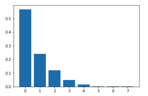
Following the Pyro code above, I tried to recreate this using:

def geometric(p, t=None):
    if t is None:
        t = 0
    x = pyro.sample("x_{}".format(t), pyro.distributions.Bernoulli(p))
    return 0 if x else 1 + geometric(p, t + 1)

# make the marginal distributions on return values explicit:
g = pyro.infer.Importance(geometric, num_samples=1000)
marginal = pyro.infer.EmpiricalMarginal(g.run(0.6))
plt.hist(marginal.sample([1000]), bins=25)

However, this raises an error in abstract_infer.py (AttributeError: ‘int’ object has no attribute ‘dtype’) for pyro.infer.EmpiricalMarginal(g.run(0.6))

Changing that line to

marginal = pyro.infer.EmpiricalMarginal(g.run(0.6), sites="x_0")

eliminates the error, but is, of course, not replicating the WebPPL example.

Clearly, I’m having trouble reconciling the conceptual differences between Pyro and WebPPL. I’m also having trouble determining exactly what the Pyro classes and functions expect and return. Reading the source helps a bit, but there are many terms that I don’t see defined and that I assume are defined in various papers. I’ve also found some older examples and blog posts that were helpful, but many of those don’t run in Pyro 0.3.

Aside from the specific issue above (can any stochastic function be turned into a first class Pyro distribution using inference?) are there any documents to explain the general concepts and nomenclature? Church/WebPPL seem very clear in contrast to Pyro.

The Importance/EmpiricalMarginal combination you’ve found is essentially equivalent to Infer({method: 'forward', ...}) in webPPL. I think your specific issue is caused by difficulties mixing PyTorch tensors and Python scalars: if you replace return 0 ... with return torch.tensor(0.) ... that error message should go away.

are there any documents to explain the general concepts and nomenclature?

There are the language intro tutorials (part 1 and part 2). If you’re interested in seeing some simple end-to-end examples ported almost line-for-line from idiomatic webPPL code, see the RSA examples (tutorial and scripts). Also, if you haven’t already, you might want to review some PyTorch tutorials, since while Pyro’s tutorials assume little or no prior knowledge of probabilistic machine learning or probabilistic programming, we do expect users to be familiar with the PyTorch tensor API.

Church/WebPPL seem very clear in contrast to Pyro.

Unfortunately, despite its elegance the idea in webPPL and Church of representing marginal distributions by building histograms of importance or random-walk MH samples doesn’t scale very well beyond the toy problems in PMC and has very bad statistical properties when used in combination with variational inference, so we don’t encourage users to do that. Current inference algorithms in Pyro instead provide you with an approximation to the joint posterior distribution over all unconstrained sample sites given all observed ones. This approximation takes different forms depending on the algorithm used, e.g. a guide program with trained parameters in SVI or a bag of samples in MCMC.

In general, Pyro is less opinionated about what you do with the approximate posterior than Church and webPPL, which actually approximate the joint posterior as a preliminary step and then aggregate return values from posterior samples into a histogram automatically.

1 Like

This indeed helps. The following code works as expected:

import torch
import pyro.infer
import pyro.distributions as dist
import numpy as np
import matplotlib.pyplot as plt
%matplotlib inline

def geometric(p, t=None):
    if t is None:
        t = 0
    x = pyro.sample("x_{}".format(t), pyro.distributions.Bernoulli(p))
    return torch.tensor(0) if x else 1 + geometric(p, t + 1)

# make the marginal distributions on return values explicit:
g = pyro.infer.Importance(geometric, num_samples=1000)
marginal = pyro.infer.EmpiricalMarginal(g.run(0.6)) # geometric(0.6)
samples = marginal.sample([1000])

labels, counts = np.unique(samples, return_counts=True, axis=0)
probs = counts/np.sum(counts)
plt.bar(range(len(labels)), probs, align='center', tick_label=[str(w) for w in labels])

My original version of geometric was based on the version in part 1 of the tutorial. It did not return a tensor, so I didn’t realize that that was a problem.

I read over tutorial part 1 and 2, but still found them somewhat confusing, perhaps because I had previously worked through PMC. For example, part 1 defines the geometric distribution as an example of the flexibility of Pyro, then later says “Pyro stochastic functions are universal, i.e., they can be used to represent any computable probability distribution.” I interpreted this to mean that I could use geometric in the same way as a built-in distribution, such as by writing:

A = pyro.sample("A", geometric(0.6))

But, of course, that doesn’t work. This raises the question of how to condition on the results of a recursive stochastic function, such as geometric, or how to use abstraction, such as by defining a flip() operator to match that in Church/WebPPL.

I’m not familiar with PyTorch, so I’ll definitely check out the tutorials before going much further with Pyro.

I interpreted this to mean that I could use geometric in the same way as a built-in distribution

Pyro’s sample primitive isn’t really any different from WebPPL’s, except that it expects a name. Think of pyro.sample as being like apply and Pyro’s distributions as being like thunks; A = dist.Geometric(0.6)() has the same default semantics outside of an inference algorithm as A = pyro.sample("A", dist.Geometric(0.6)). Just as in WebPPL, you’re free to use your function geometric inside other functions in the usual way, or construct its marginal and use that with pyro.sample just like dist.Geometric.

This raises the question of how to condition on the results of a recursive stochastic function, such as geometric

Here’s an old GitHub discussion about expressing arbitrary constraints. However, there are fundamental computational limits on the sort of query you can compute in any PPL. Consider the following Pyro program:

def magic():
    assignment = [pyro.sample("value_{}".format(i), Bernoulli(0.5)) for i in range(k)]
    pyro.sample("satisfied", some_CNF_formula, assignment, obs=True)
    return assignment

Computing the marginal distribution over its return values is equivalent to counting the number of satisfying assignments to some_CNF_formula, which is #P-complete. In fact, because languages like Pyro and Church are so expressive, there are even more pathological cases: there exist computable random variables and constraints whose posterior is not computable.

Confronted with such severe intractability, inference algorithms in PPLs are designed for problems whose solutions we know how to approximate, meaning that only some of the programs we can write down are compatible with currently implemented inference algorithms. In Pyro, this means programs to whose executions we can assign positive (unnormalized) probability densities; as a result, inference algorithms expect the input to pyro.sample to have a log_prob method that assigns a finite score to any output value. Soft constraints (equivalent to factor in WebPPL) are expressed in the form of observed output values for pyro.sample statements.

The program above is not compatible with any of Pyro’s current inference algorithms because we’d have to solve a k-SAT instance to find any execution with positive probability, although it can be modified slightly so that it is as discussed in the GitHub issue above. The examples in PMC with hard constraints are thus a little misleading in the sense that existing PPLs can only handle very small/simple instances of such problems, although this is an area of ongoing research.