I’m playing around with a toy problem, representative of a real problem I’m trying to solve. Say we have a canon positioned to fire a projectile at some angle and velocity and we can measure the resulting trajectory. The canon has a wobble or something so the initial angle and velocity are uncertain. I’m trying to infer the uncertainty in both by observing a number of trajectories.
The working code below simulates some number of trajectories using known normal distributions for the angle and velocity. For compatibility with my actual problem the trajectories are stored as a n_time x n_batch x 2 tensor. The code then runs a MAP estimate for the mean values of the actual distributions and then SVI to try to find both the mean and variance.
The MAP estimate is fine, with these settings it recovers the mean of the input distributions. SVI again recovers the mean but, as the final plots that the code generates shows, the estimate of the variance of both the angle and velocity distributions is too low. This is very consistent no matter how I set the prior or the initial (AutoNormal) scale parameters. For example, even if I set the initial guide variances to be high the inference process will still tend to send them towards zero.
Is there something fundamentally wrong with this approach or does anyone have any suggestions on how to improve the variance predictions?
import numpy as np
import matplotlib.pyplot as plt
import torch
import pyro
import pyro.distributions as dist
from pyro.contrib.autoguide import AutoDiagonalNormal, AutoDelta, AutoNormal, init_to_mean
from pyro.infer import SVI, Trace_ELBO, Predictive
import pyro.optim as optim
from tqdm import tqdm
g = torch.tensor(0.1)
v_loc_act = 2.0
v_scale_act = 0.1
a_loc_act = np.pi/6.0
a_scale_act = 0.02
v_loc_prior = 1.5
v_scale_prior = 0.2
a_loc_prior = np.pi/4
a_scale_prior = 0.04
eps = 1.0e-4
pyro.enable_validation()
def model_act(times):
"""
times: ntime x nbatch
trajectories: ntime x nbatch x 2
"""
v = pyro.sample("v", dist.Normal(v_loc_act, v_scale_act))
a = pyro.sample("a", dist.Normal(a_loc_act, a_scale_act))
simulated = torch.stack((
v * torch.cos(a) * times,
v * torch.sin(a) * times - 0.5 * g * times**2.0)).T
return simulated
def model(times, actual = None):
"""
times: ntime x nbatch
trajectories: ntime x nbatch x 2
"""
v = pyro.sample("v", dist.Normal(v_loc_prior, v_scale_prior))
a = pyro.sample("a", dist.Normal(a_loc_prior, a_scale_prior))
simulated = torch.stack((
v * torch.cos(a) * times,
v * torch.sin(a) * times - 0.5 * g * times**2.0)).permute((1,2,0))
with pyro.plate("trials", times.shape[1]):
with pyro.plate("time", times.shape[0]):
pyro.sample("obs", dist.Normal(simulated, eps).to_event(1), obs = actual)
return simulated
if __name__ == "__main__":
nsamples = 50
tmax = 20.0
tnum = 100
time = torch.linspace(0, tmax, tnum)
times = torch.empty(tnum, nsamples)
data = torch.empty(tnum, nsamples, 2)
with torch.no_grad():
for i in range(nsamples):
times[:,i] = time
data[:,i] = model_act(time)
plt.plot(data[:,:,0], data[:,:,1])
plt.show()
# MAP
print("MAP")
pyro.clear_param_store()
lr = 1.0e-3
niter = 1250
num_samples = 1
guide = AutoDelta(model, init_loc_fn = init_to_mean())
optimizer = optim.Adam({"lr": lr})
svi = SVI(model, guide, optimizer,
loss = Trace_ELBO(num_particles=num_samples))
t = tqdm(range(niter))
loss_hist = []
for i in t:
loss = svi.step(times, data)
loss_hist.append(loss)
t.set_description("Loss: %3.2e" % loss)
print("MAP velocity: %4.3f, actual %4.3f" % (pyro.param("AutoDelta.v").data,
v_loc_act))
print("MAP angle: %4.3f, actual %4.3f" % (pyro.param("AutoDelta.a").data,
a_loc_act))
plt.semilogy(loss_hist)
plt.show()
print("")
# Inference with AutoNormal
pyro.clear_param_store()
print("AutoNormal")
lr = 1.0e-3
niter = 8000
num_samples = 5
guide = AutoNormal(model, init_loc_fn = init_to_mean(),
init_scale = 0.1)
# Initialize the guide
guide(times, data)
optimizer = optim.Adam({"lr": lr})
svi = SVI(model, guide, optimizer,
loss = Trace_ELBO(num_particles=num_samples))
print("Start:")
print("Velocity mean: %4.3f, actual %4.3f" % (pyro.param("AutoNormal.locs.v").data,
v_loc_act))
print("Velocity scale: %4.3f, actual %4.3f" % (pyro.param("AutoNormal.scales.v").data,
v_scale_act))
print("Angle mean: %4.3f, actual %4.3f" % (pyro.param("AutoNormal.locs.a").data,
a_loc_act))
print("Angle scale: %4.3f, actual %4.3f" % (pyro.param("AutoNormal.scales.a").data,
a_scale_act))
t = tqdm(range(niter))
loss_hist = []
for i in t:
loss = svi.step(times, data)
loss_hist.append(loss)
t.set_description("Loss: %3.2e" % loss)
print("Inference:")
print("Velocity mean: %4.3f, actual %4.3f" % (pyro.param("AutoNormal.locs.v").data,
v_loc_act))
print("Velocity scale: %4.3f, actual %4.3f" % (pyro.param("AutoNormal.scales.v").data,
v_scale_act))
print("Angle mean: %4.3f, actual %4.3f" % (pyro.param("AutoNormal.locs.a").data,
a_loc_act))
print("Angle scale: %4.3f, actual %4.3f" % (pyro.param("AutoNormal.scales.a").data,
a_scale_act))
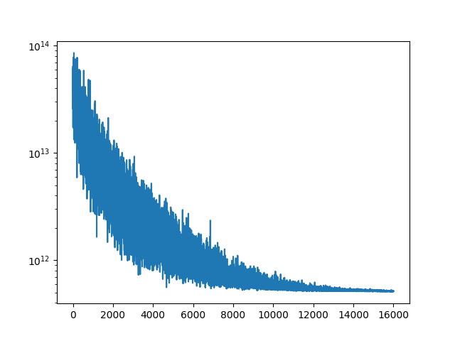
plt.semilogy(loss_hist)
plt.show()
nsample = 200
predict = Predictive(model, guide = guide, num_samples = nsample,
return_sites=("obs",))
with torch.no_grad():
samples = predict(times[:,0:1])["obs"][:,:,0]
min_x, _ = torch.min(samples[:,:,0], 0)
max_x, _ = torch.max(samples[:,:,0], 0)
min_y, _ = torch.min(samples[:,:,1], 0)
max_y, _ = torch.max(samples[:,:,1], 0)
plt.plot(times, data[:,:,1], 'k-', lw = 0.1)
plt.fill_between(time, min_y, max_y, alpha = 0.75)
plt.show()
plt.plot(times, data[:,:,0], 'k-', lw = 0.1)
plt.fill_between(time, min_x, max_x, alpha = 0.75)
plt.show()