Independent priors and correlated posteriors

[3mtmuhPnQv]

Suppose I have a 2-dimensional vector of linear model coefficients with independent Normal(0, 1) priors

theta = pyro.sample('theta', dist.Normal(torch.zeros(3), torch.ones(3)).to_event(1))
sigma = pyro.sample('sigma', dist.LogNormal(0, 1))
mu = torch.matmul(X, theta)
pyro.sample('obs', dist.Normal(mu, sigma), obs=y)

Is it safe to instead do

with pyro.plate("theta_plate", 3):
    theta = pyro.sample("theta", Normal(0, 1))  # .expand([10]) is automatic
    sigma = pyro.sample('sigma', dist.LogNormal(0, 1))
    mu = torch.matmul(X, theta)
    pyro.sample('obs', dist.Normal(mu, sigma), obs=y)

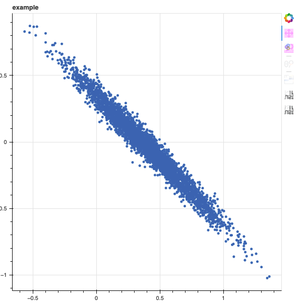
While the priors for each theta value are independent, the posterior for the theta values can still have correlation introduced by the likelihood. For example, if the columns of X are highly multicollinear.

I guess my fundamental question is what is pyro doing under the hood with plates? I’m having trouble understanding the precise meaning of the different independences. I’m coming from Stan, so I understand probabilistic modeling as specifying the joint log probability of any particular n-tuple of parameters, then running some kind of exploration algorithm over potential parameter tuples. What does it actually do to the log probability of a set of parameters when you run .to_event(1) vs looping over a plate?

[martinjankowiak]

what happens under the hood depends on the inference algorithm. can you maybe formulate a more precision question?

note that if you’re unsure about sample shapes and such it can be useful to add lots of assert statements, e.g.

with pyro.plate("theta_plate", 3):
    theta = pyro.sample("theta", Normal(0, 1))
    assert theta.shape == (...)

[3mtmuhPnQv]

My precise question is whether or not it’s safe to replace this

theta = pyro.sample('theta', dist.Normal(torch.zeros(3), torch.ones(3)).to_event(1))
sigma = pyro.sample('sigma', dist.LogNormal(0, 1))
mu = torch.matmul(X, theta)
pyro.sample('obs', dist.Normal(mu, sigma), obs=y)

with this

with pyro.plate("theta_plate", 3):
    theta = pyro.sample("theta", Normal(0, 1))  # .expand([10]) is automatic
    sigma = pyro.sample('sigma', dist.LogNormal(0, 1))
    mu = torch.matmul(X, theta)
    pyro.sample('obs', dist.Normal(mu, sigma), obs=y)

Are these the same probability model, particularly in the case where I have independent priors on theta but correlation is induced in the posterior by the likelihood?

To illustrate what I mean, here’s an example of a very simple quadratic regression with independent priors and correlated posteriors on the coefficients.

import os
import itertools
import scipy as scp
from scipy import stats as st
import numpy as np
import pandas as pd
import cmdstanpy as stn
from bokeh import plotting as bpl
from bokeh import io as bio
bio.output_notebook()

model_code = """
data {
    int N;
    matrix[N, 2] X;
    vector[N] y;
}
parameters {
    real intercept;
    vector[2] theta;
    real<lower=0> sigma;
}
transformed parameters {
    vector[N] y_hat = X * theta + intercept;
}
model {
    theta ~ normal(0, 1);
    intercept ~ normal(0, 1);
    sigma ~ student_t(3, 0, 1);
    y ~ normal(y_hat, sigma);
}   
"""
def compile_model(filename, model_code):
    stanfile_name = f'{filename}.stan'
    rewrite = True
    if os.path.exists(stanfile_name):
        with open(stanfile_name, 'r') as f:
            current_code = f.read()
        rewrite = current_code != model_code
    if rewrite:            
        with open(stanfile_name, 'w') as f:
            f.write(model_code)
    return stn.CmdStanModel(stan_file=stanfile_name)

stanmodel = compile_model('test_model', model_code)

N = 10000
x = np.expand_dims(np.random.uniform(-1, 1, N), axis=1)
intercept = 0.65
theta = np.array([0.1, 0.2])
sigma = 3.0
X = np.concatenate((x, np.random.normal(x, 0.1)), axis=1)
mu = intercept + np.matmul(X, theta)
y = np.random.normal(mu, sigma)

fit = stanmodel.sample(
    data={
        'N': N,
        'X': X,
        'y': y,
    },
)

fit_dict = fit.stan_variables()
theta_draws = fit_dict['theta']
intercept_draws = fit_dict['intercept']
sigma_draws = fit_dict['sigma']
fit_df = pd.DataFrame({
    'intercept': intercept_draws,
    'theta_0': theta_draws[:,0],
    'theta_1': theta_draws[:,1],
    'sigma_draws': sigma_draws,
})
fig = bpl.figure(title='example')
fig.circle(x=fit_df['theta_0'].values, y=fit_df['theta_1'].values)
bio.show(fig)

The collinearity of the two regressors induces a very distinct anti-correlation in their joint posterior distribution, even though their priors are independent.

[3mtmuhPnQv]

More generally, the documentation says this

Indices over .batch_shape denote conditionally independent random variables, whereas indices over .event_shape denote dependent random variables (ie one draw from a distribution).

But I’m not sure what probability model they’re talking about. Data are typically independent random variables conditional on particular parameters in their generative model. But in the probability model for those parameters, data aren’t random variables at all, only the parameters, which can be independent in their priors but not independent in their posteriors. My view of probabilistic programming, biased by having started with stan, is that you have some sample space of parameters you’re interested in, some way to define the log probability of any parameters tuple, and some exploration algorithm (NUTS, SVI, etc) that traverses that log probability landscape to produce a representative set of potential parameter values. I’d be more comfortable interpreting these documents if I knew how exactly a set of pyro.sample calls defines that joint log probability in parameter space.

[martinjankowiak]

@3mtmuhPnQv

sigma = pyro.sample('sigma', dist.LogNormal(0, 1))

if you put this sample statement in a plate context it will be automatically expanded to the size of the plate. i’m assuming that’s not what you want? again, i suggest the use of assert statements to make sure you get samples of the expected shape.

it’s a bit difficult to make general statements in this context because the details depend on the inference algorithm. the model defines a joint probability density, yes. in principle if you give me a joint density that i can, say, evaluate pointwise i could figure out the conditional independence structure (although doing so may be difficult). however that conditional independence will not be manifest. to make that conditional independence manifest pyro uses plate contexts (another option would be to do static analysis of python code to determine conditional indepencies; but that’s messy/complex). this information is then available to inference algorithms.

if you run HMC/NUTS on a model with only continuous latent variables this information is irrelevant. HMC/NUTS doesn’t make use of conditional independence information. all it needs is gradients of the log joint density. in particular plates will not change the posterior samples generated.

if, however, the model includes discrete latent variables the conditional independence structure may well matter. in stan (unless you explicitly sum out the discrete latent variables by hand) you’re out of luck in this setting. by contrast pyro will sum out the discrete latent variables if doing so is tractable. that tractability in turn depends on the conditional independence structure. treewidth and what not.

similar points could be made about variational inference. plates in the model can, for example, have a substantial impact on the ELBO gradient estimators that are constructed in the presence of discrete latent variables (keyword: rao-blackwellization). similarly plates in the guide can be used to make conditional independence assumptions in the variational family manifest. that will, of course, have an impact on the approximately variational distribution learned.

and the details go on and on since the world of inference algorithms goes on and on and on