I am making a comparison between Dan Foreman Mackey’s “Astronomer’s Guide to NumPyro”, attempting to demonstrate how SVI can be used to approach his first example of “linear relationships with outliers” as an alternative to MCMC. I have tried three different approaches:
- An autoguide using
AutoMultivariateNormal - An autoguide using
AutoNormal/AutoDiagonalNormal - A manually defined uncorrelated normal guide
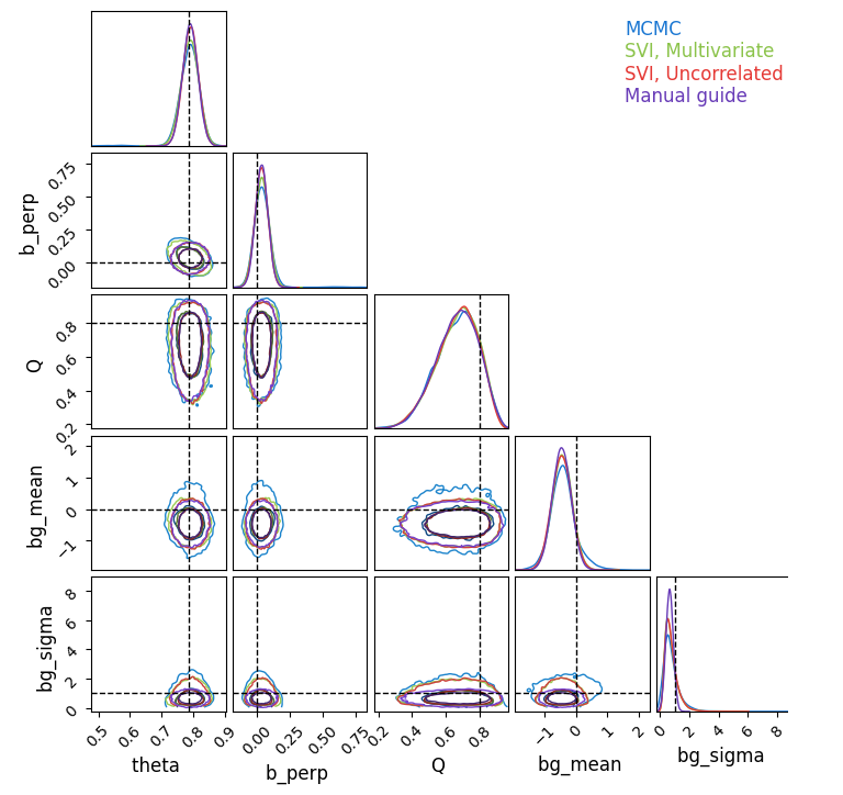
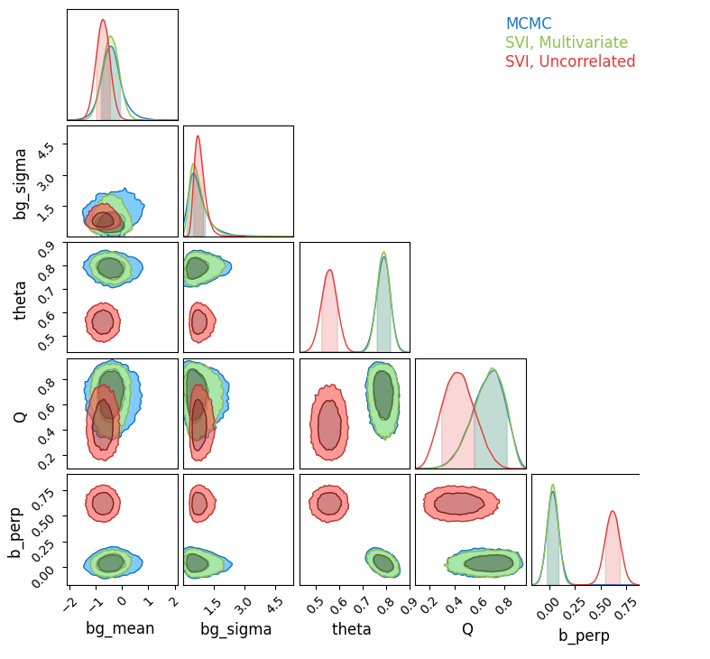
I am getting good results (in agreement with MCMC) for option 1, but not for option 2, even though the true posterior is not strongly correlated (see below). Option 3 is failing entirely, diverging to nan loss results. This may be a result of issues with constrained / unconstrained domains, but I’m surprised to see it breaking so easily. I have included snippets of code and an outline of the model below.
I am most concerned with the issues presented by the uncorrelated autoguide. Have I implemented this correctly?
Likelihood Contours for MCMC and Autoguides
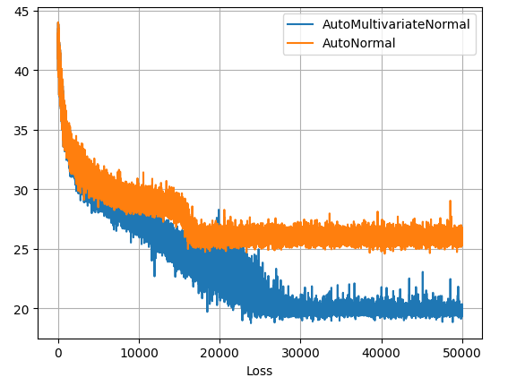
I can confirm that the SVI runs are fully converged from their loss-plots plateauing, though the uncorrelated surrogate model is obviously leveling out at a worse fit.
Model
The model is a direct copy of DFM’s code, minus the commenting. It is a mixture model of time series measurements with gaussian error fitted to a mixture of a linear relationship and a normally distributed background. The slope and offset of the line are re-parameterized in terms of slope angle \theta rather than gradient m=\text{tan}(\theta):
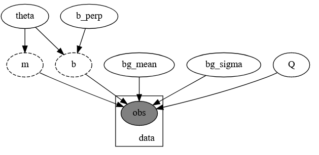
Model PGM
Model Example From DFM
# Model
def linear_mixture_model(x, yerr, y=None):
# Angle & offset of linear relationship
theta = numpyro.sample("theta", dist.Uniform(-0.5 * jnp.pi, 0.5 * jnp.pi))
b_perp = numpyro.sample("b_perp", dist.Normal(0.0, 1.0))
# Linear relationship distribution
m = numpyro.deterministic("m", jnp.tan(theta))
b = numpyro.deterministic("b", b_perp / jnp.cos(theta))
fg_dist = dist.Normal(m * x + b, yerr)
# Pure normally distributed background for outliers
bg_mean = numpyro.sample("bg_mean", dist.Normal(0.0, 1.0))
bg_sigma = numpyro.sample("bg_sigma", dist.HalfNormal(3.0))
bg_dist = dist.Normal(bg_mean, jnp.sqrt(bg_sigma**2 + yerr**2))
# Mixture of linear foreground / w background
Q = numpyro.sample("Q", dist.Uniform(0.0, 1.0)) # Relative weighting of foreground & background
mix = dist.Categorical(probs=jnp.array([Q, 1.0 - Q])) # Categorical distribution = each sample has a weighted chance of belonging to each category
# Using mixture distribution, measure likelihood of all observations
with numpyro.plate("data", len(x)):
numpyro.sample("obs", MixtureGeneral(mix, [fg_dist, bg_dist]), obs=y)
#--------------------------------------------------------
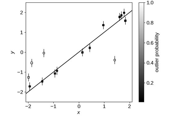
# Data Generation
true_frac = 0.8 # Fraction of outliers
true_params = [1.0, 0.0] # slope & offset of linrel
true_outliers = [0.0, 1.0] # mean and sigma of background
# Generate data
np.random.seed(12)
x = np.sort(np.random.uniform(-2, 2, 15))
yerr = 0.2 * np.ones_like(x)
y = true_params[0] * x + true_params[1] + yerr * np.random.randn(len(x))
# Shuffle outliers
m_bkg = np.random.rand(len(x)) > true_frac # select these elements to re-sample from bg dist
y[m_bkg] = true_outliers[0]
y[m_bkg] += np.sqrt(true_outliers[1] + yerr[m_bkg] ** 2) * np.random.randn(sum(m_bkg))
Manual Guide Definition
def manual_guide(x, yerr, y):

    #------------------------------
    # Distribution Means

    bg_mean_mu = numpyro.param('bg_mean_mu', 0.0, constraint =constraints.real)
    bg_sigma_mu = numpyro.param('bg_sigma_mu', 1.0, constraint =constraints.positive)
    theta_mu = numpyro.param('theta_mu', jnp.pi / 4, constraint =constraints.interval(-jnp.pi/2, jnp.pi/2))
    Q_mu = numpyro.param('Q_mu', 0.8, constraint =constraints.unit_interval)
    b_perp_mu = numpyro.param('bg_perp_mu', 0.0, constraint =constraints.real)

    #------------------------------
    # Distribution Variances
    bg_mean_sigma = numpyro.param('bg_mean_mu', 0.01, constraint =constraints.positive)
    bg_sigma_sigma = numpyro.param('bg_sigma_sigma', 0.01, constraint =constraints.positive)
    theta_sigma = numpyro.param('theta_sigma', 0.01, constraint =constraints.positive)
    Q_sigma = numpyro.param('Q_mu', 0.01, constraint =constraints.positive)
    b_perp_sigma = numpyro.param('bg_perp_mu', 0.01, constraint =constraints.positive)

    #------------------------------
    # Construct & Sample Distributions
    numpyro.sample('bg_mean', dist.Normal(bg_mean_mu, bg_mean_sigma))
    numpyro.sample('bg_sigma', dist.Normal(bg_sigma_mu, bg_sigma_sigma))
    numpyro.sample('theta', dist.Normal(theta_mu, theta_sigma))
    numpyro.sample('Q', dist.Normal(Q_mu, Q_sigma))
    numpyro.sample('b_perp', dist.Normal(b_perp_mu, b_perp_sigma))
Autoguide Generation & SVI Optimization
optimizer_forauto = numpyro.optim.Adam(step_size=0.00025)

autoguy = numpyro.infer.autoguide.AutoMultivariateNormal(linear_mixture_model)
autoguysvi = SVI(linear_mixture_model, autoguy, optim = optimizer_forauto, loss=Trace_ELBO(num_particles=8))

autoguy_diag = numpyro.infer.autoguide.AutoDiagonalNormal(linear_mixture_model)
autoguysvi_diag = SVI(linear_mixture_model, autoguy_diag, optim = optimizer_forauto, loss=Trace_ELBO(num_particles=8))

manual_guide_svi = SVI(linear_mixture_model, manual_guide, optim = optimizer_forauto, loss=Trace_ELBO(num_particles=8))

autoguysvi_result = autoguysvi.run(random.PRNGKey(2), 50000, x, yerr, y=y)
autoguysvi_result_diag = autoguysvi_diag.run(random.PRNGKey(2), 50000, x, yerr, y=y)
manual_guide_svi_result = manual_guide_svi.run(random.PRNGKey(2), 50000, x, yerr, y=y)
Sample Retrieval & Plotting
res = sampler.get_samples()

c = ChainConsumer()
c.add_chain(res, name="MCMC")

svi_pred = Predictive(autoguy, params = autoguysvi_result.params, num_samples = 20000*2)(rng_key = jax.random.PRNGKey(1))
svi_pred.pop('_auto_latent')
svi_pred_diag = Predictive(autoguy_diag, params = autoguysvi_result_diag.params, num_samples = 20000*2)(rng_key = jax.random.PRNGKey(1))
svi_pred_diag.pop('_auto_latent')

c.add_chain(svi_pred, name="SVI, Multivariate")
c.add_chain(svi_pred_diag, name="SVI, Uncorrelated")
c.plotter.plot(parameters = {'theta', 'b_perp', 'Q', 'bg_mean', 'bg_sigma'})

plt.show()