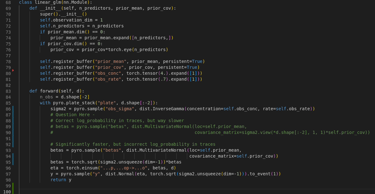
Hi @fritzo, thanks for the response! I completely agree that the models are distributionally equivalent but semantically different. But I guess my question is: is it possible to make them semantically equivalent within pyro? So for a concrete example lets say we wanted to calculate the marginal prior entropy of the “beta” parameters.
import torch
import pyro
from pyro import poutine
import pyro.distributions as dist
from pyro.contrib.util import lexpand
import math

n_predictors = 5
n_subjects = 7
n_designs = 25
prior_mean = torch.zeros(n_predictors)
prior_cov = 5. * torch.eye(n_predictors)
prior_concentration = 3
prior_rate = 1

designs = torch.randn(n_designs, n_subjects, n_predictors)


def slow_linear_model_correct_traces(d):
    with pyro.plate_stack("plate", d.shape[:-2]):
        sigma2 = pyro.sample("obs_sigma", dist.InverseGamma(concentration=prior_concentration, rate=prior_rate))
        betas = pyro.sample("betas", dist.MultivariateNormal(loc=prior_mean,
                                                             covariance_matrix=sigma2.view(*d.shape[:-2], 1, 1)*prior_cov))
        eta = torch.einsum("...p,...op->...o", betas, d)
        y = pyro.sample("y", dist.Normal(eta, torch.sqrt(sigma2.unsqueeze(dim=-1))).to_event(1))
        return y

def fast_linear_model_incorrect_traces(d):
    with pyro.plate_stack("plate", d.shape[:-2]):
        sigma2 = pyro.sample("obs_sigma", dist.InverseGamma(concentration=prior_concentration, rate=prior_rate))
        betas = pyro.sample("betas", dist.MultivariateNormal(loc=prior_mean,
                                                             covariance_matrix=prior_cov))
        betas = torch.sqrt(sigma2.unsqueeze(dim=-1))*betas
        eta = torch.einsum("...p,...op->...o", betas, d)
        y = pyro.sample("y", dist.Normal(eta, torch.sqrt(sigma2.unsqueeze(dim=-1))).to_event(1))
        return y

def empirical_prior_entropy(model, designs):
    N = 500
    M = 50
    expanded_designs = lexpand(designs, N)
    trace = poutine.trace(model).get_trace(expanded_designs)

    conditoned_model = poutine.condition(model, {"betas": trace.nodes["betas"]["value"]})
    reexpanded_designs = lexpand(expanded_designs, M)
    retrace = poutine.trace(conditoned_model).get_trace(reexpanded_designs)
    retrace.compute_log_prob()
    prior_entropy = -1*(retrace.nodes["betas"]["log_prob"].logsumexp(dim=0) - math.log(M)).mean(dim=0)
    return prior_entropy

# Analytic Calculation of Prior Entropy
marginal_prior_cov = (prior_rate/prior_concentration) * prior_cov
prior_entropy = torch.distributions.StudentT(df=2*prior_concentration, loc=prior_mean, scale=torch.ones(n_predictors)).entropy().sum() \
                    + 0.5*torch.log(torch.det(marginal_prior_cov))
print(f"Analytic Prior Entropy {prior_entropy}")
# Analytic Prior Entropy 9.235673904418945

print(empirical_prior_entropy(slow_linear_model_correct_traces, designs).mean())
# Output: tensor(9.1409) - Correct
print(empirical_prior_entropy(fast_linear_model_incorrect_traces, designs).mean())
# Output tensor(11.1133) - Incorrect
We can see that the model that doesn’t reparameterize the beta parameters achieves the correct result, whereas this is not the case for the model that does reparamterize. Unfortunately there is also a significant speed difference as well.
Is it possible to keep the reparmaterization in the fast approach while still having the trace.nodes[“betas”[“log_prob”] remain correct?
Sorry about the screenshot, I’ll make sure to include the code in markdown from now on.