How to try gradient-free sampler for Lotka-Volterra example?

I’m new to numpyro but have used pymc and diffrax/JAX. I’m adapting the numpyro Lotka-Volterra ODE tutorial to use the JAX package diffrax that is officially recommended instead of odeint: Example: Predator-Prey Model — NumPyro documentation

Here’s my simple code rewriting that tutorial…

from jax import config
config.update("jax_enable_x64", True)
from jax.random import PRNGKey
import jax.numpy as jnp
from jax import jit
import numpyro
import numpyro.distributions as dist
from numpyro.examples.datasets import LYNXHARE, load_dataset
from numpyro.infer import MCMC, NUTS, Predictive
from diffrax import diffeqsolve, ODETerm, SaveAt, Tsit5

### download pre-packaged numpyro data for Lotka-Volterra problem
_, fetch = load_dataset(LYNXHARE, shuffle=False)
year, data = fetch()  # data is in hare -> lynx order

### Lotka-Volterra ODE function
def vector_field(t, y, args):
    prey, predator = y
    alpha, beta, gamma, delta = args    
    dprey_dt = alpha * prey - beta * prey * predator
    dpredator_dt = -gamma * predator + delta * prey * predator
    return dprey_dt, dpredator_dt

### setup for diffrax
term = ODETerm(vector_field)
solver = Tsit5()
t0 = jnp.asarray(year[0],dtype=jnp.float64)
t1 = jnp.asarray(year[-1],dtype=jnp.float64)
dt0 = 0.1 
y0 = (20,30)
args = (0.52, 0.026, 0.84, 0.026) 
saveat = SaveAt(ts=jnp.asarray(year,dtype=jnp.float64)) # evaluate at same times as observations

### jitted function that solves ODE for given initial conditions (y0) and free parameters (args)
@jit
def solve_diffrax(y0,args):
    # returning transposed solution so it has same dims as data: 91x2
    return jnp.asarray(diffeqsolve(term, solver, t0, t1, dt0, y0, args=args, saveat=saveat).ys).T

def model(obs_data):
    
    init_hare = numpyro.sample("init_hare", dist.LogNormal(jnp.log(10), 1)) # mean-log(10), sigma=1
    init_lynx = numpyro.sample("init_lynx", dist.LogNormal(jnp.log(10), 1))
    y_init = (init_hare, init_lynx)

    alpha = numpyro.sample('alpha',dist.TruncatedNormal(low=0.0,loc=1.0,scale=0.5))
    beta = numpyro.sample('beta',dist.TruncatedNormal(low=0.0,loc=0.05,scale=0.05))
    gamma = numpyro.sample('gamma',dist.TruncatedNormal(low=0.0,loc=1.0,scale=0.5))
    delta = numpyro.sample('delta',dist.TruncatedNormal(low=0.0,loc=0.05,scale=0.05))    
    theta = (alpha,beta,gamma,delta)
    
    # get diffrax solution for current parameters (evaluated at same times as observations)
    sol = solve_diffrax(y_init,theta)
    
    sigma = numpyro.sample("sigma", dist.LogNormal(-1, 1).expand([2]))    
    
    numpyro.sample("y", dist.LogNormal(jnp.log(sol), sigma), obs=obs_data)

### finally do the same call as in numpyro example
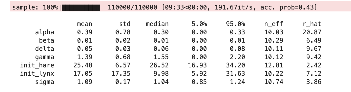
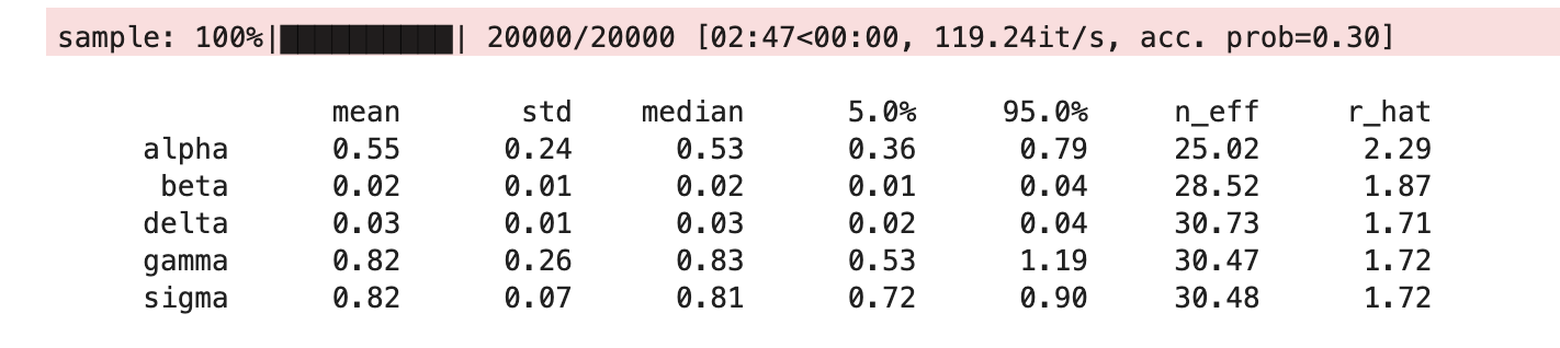
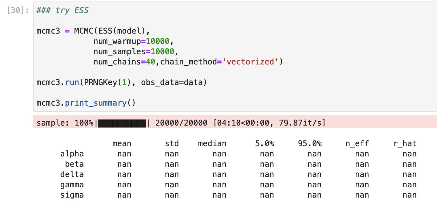
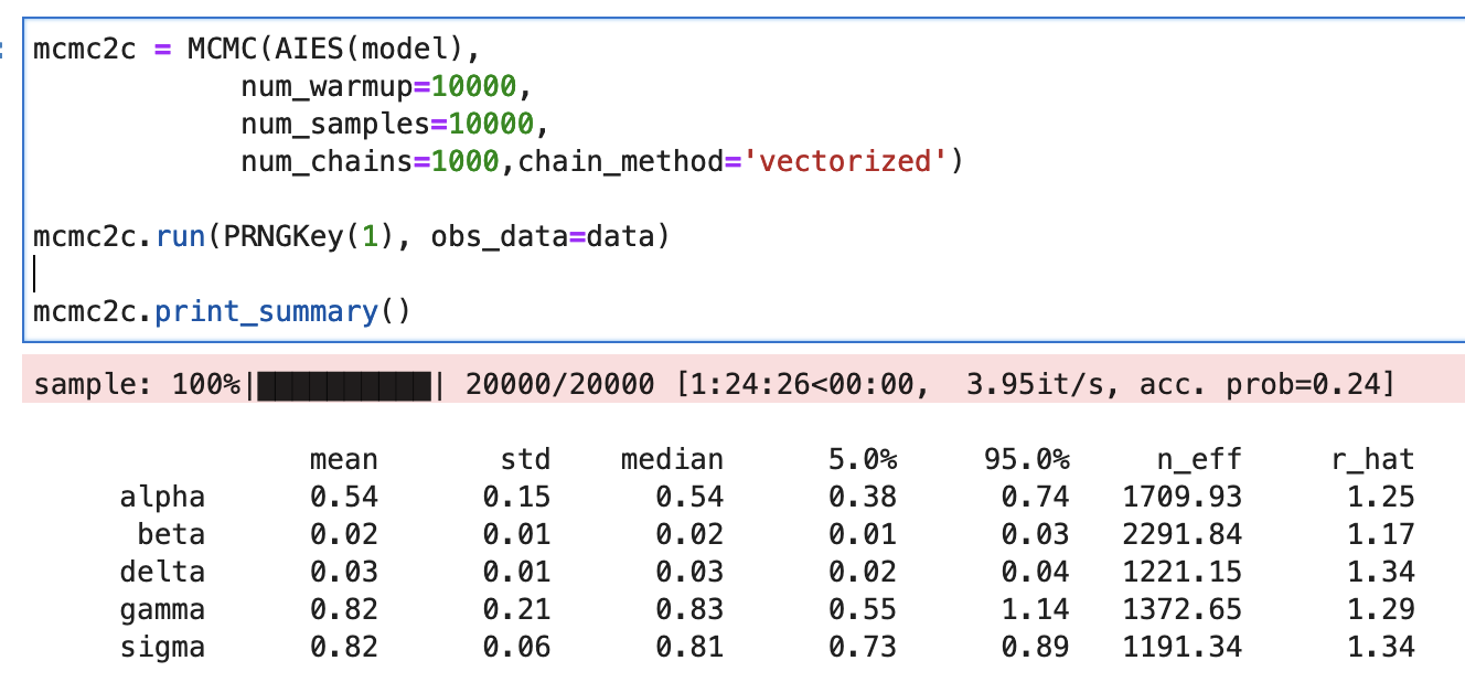
###### How do I use a gradient-free (non-NUTS) approach?
mcmc = MCMC(NUTS(model, dense_mass=True),
            num_warmup=1000,
            num_samples=1000,
            num_chains=1)

mcmc.run(PRNGKey(1), obs_data=data)

It works with NUTS but now I want to try with a gradient-free sampler for comparison. How do I change the second to last line (mcmc = MCMC(NUTS(models...))) to use a gradient-free sampler and which gradient-free samplers are recommended/available for this kind of problem?

hard to say what gradient-free methods, if any, will work well but you can try

https://num.pyro.ai/en/latest/mcmc.html#numpyro.infer.ensemble.AIES
https://num.pyro.ai/en/latest/mcmc.html#numpyro.infer.ensemble.ESS
https://num.pyro.ai/en/latest/mcmc.html#numpyro.infer.sa.SA

Well I got it sampling with AIES but the r-hat is terrible even with 100K warmup and 10K samples:

mcmc2 = MCMC(AIES(model),
            num_warmup=100000,
            num_samples=10000,
            num_chains=20,chain_method='vectorized')

mcmc2.run(PRNGKey(1), obs_data=data)

mcmc2.print_summary()

Any idea what else to try? I don’t necessarily want to use this for actual constraints but rather to do a comparison of how fast NUTS converges vs. how long a gradient-free sampler would take. Given enough warmup, AIES or the other gradient-free samplers SHOULD cover the parameter space, no?

The acceptance probability is also pretty low: ~40% in AIES vs. ~90% for NUTS.

given the low dimensionality it should probably work with gradient-free methods given enough samples. i haven’t much intuition about good hyperparameters etc for ESS/AIES but @amifalk would know

@quantumdoodle I would say an acceptance probability between 20 and 40% is fairly typical for something like AIES - it is not known for being terribly sample efficient (though each sample only requires one likelihood evaluation to compute and it scales well with large number of chains on gpu). ESS, being a slice sampler, tends to have a much larger effective sample size if it mixes well and can explore the full space, but YMMV there. In general, I don’t expect you to do much better than with the default arguments without heavy tweaking and experimentation; one of the nice aspects of AIES is that what you see is often what you get in terms of sampler performance.

For better results (for both AIES and ESS), you might try increasing the number of chains, initializing near a region of high posterior density, and thinning the posterior samples. 100k warmup samples strikes me as far too many given that we don’t do anything special during warmup, but it’s hard to say not having worked on your particular problem. You can check whether your chains have achieved pseudo-convergence by the end of the warmup period by collecting the warmup samples and examining their log likelihood values.

Thanks @martinjankowiak @amifalk

So I simplified the gradient-free problem a bit by fixing the initial conditions y0=(50,30) based on the NUTS result. This just cuts down the dimensionality of the problem since doing inference for ODEs is challenging. Then I am only trying to infer alpha, beta, gamma, delta and a single uncertainty sigma for the solution (# hares and lynxes vs time).

AIES does a bit better with chains=40 and 10K warmup + 10K samples – the parameter means and std’s are all close to the NUTS results and the rhat’s are all closer to 1:

However ESS gives all NaN’s – any ideas?

i have no idea but it may be some issue with your invocation of diffrax (tolerance?) or the specific form of your model (truncated normal prior with small scale? what happens for sol → 0? etc)

I will also say that I have experienced ESS in particular and to a certain extent SA to be numerically instable for difficult geometries. For ESS, you could try setting init_mu to a smaller number and turning off tune_mu to decrease the size of each slice sampling “stepping in” and “stepping out” step, though it may be that ESS is just a poor fit for this problem.

Thanks @martinjankowiak @amifalk So it seems AIES is doing well with much larger num_chains=500 or 1000 but keeping warmup=samples=10K each:

Results agree with NUTS but take ~45 min (500 chains) or ~90 min (1000 chains) vs. just ~5 min for NUTS. The AIES run uses chain_method=‘vectorized’ – I guess if ‘parallel’ was an option it’d be even faster since I have 60 CPU cores? I guess the rhat could be closer to 1 but I’d say it’s more or less converged – maybe increasing num_warmup or num_samples would help?

I have not tried to get ESS/SA to work – those are running on the exact same model/priors so it must be something else that is weirdly leading to NaN’s…