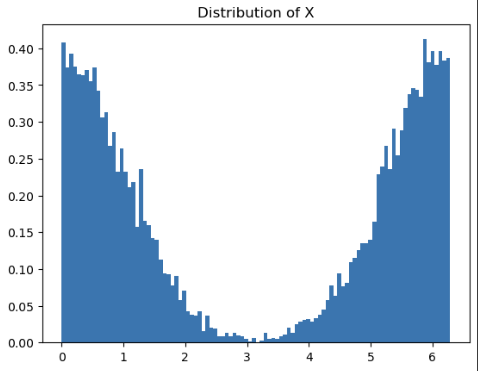
I am attempting to construct a normalizing flow that effectively transforms a base standard normal distribution into a multimodal distribution of a random variable X. This variable X is defined as follows:
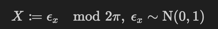
The resulting distribution of X is shown below:
I am looking to determine if it’s feasible to approximate this modulo operator using a normalizing flow. I have employed the spline_coupling transform, as used in the Pyro tutorial, but the outcome suggests it may not have sufficient flexibility to capture the multimodal nature of X’s distribution.
Here is the code I’ve been working with:
# define transform from eps_x to X
import pyro.distributions.transforms as T
import pyro.distributions as dist
eps_x_distribution = dist.Normal(torch.zeros(1), torch.ones(1))

spline_transform = T.spline_coupling(1, count_bins=16) # this transform doesn't work
flow_dist = dist.TransformedDistribution(eps_x_distribution, [spline_transform])

# and then.. need to "train" based on "actual observations"
steps = 1000
X_obs = torch.tensor(X, dtype=torch.float) # X is output of modulo operation
print(X_obs.shape)
X_obs = torch.tensor(X, dtype=torch.float).unsqueeze(-1)
print(X_obs.shape)
optimizer = torch.optim.Adam(spline_transform.parameters(), lr=1e-2) # spline transform from T.Spline
for step in range(steps):
    optimizer.zero_grad()
    loss = -flow_dist.log_prob(X_obs).mean() # nll
    loss.backward()
    optimizer.step()
    flow_dist.clear_cache()

    if step % 200 == 0:
        print('step: {}, loss: {}'.format(step, loss.item()))

# Generate samples from the eps_x distribution
eps_x_samples = eps_x_distribution.sample(sample_shape=torch.Size([10000, 1]))

# Apply the learned spline transform to the samples
X_samples = spline_transform(eps_x_samples)

# Plot the transformed samples
plt.hist(X_samples.detach().numpy().squeeze(), bins=100, density=True, alpha=0.5, label='Transformed samples')

# Plot the actual observed data
plt.hist(X_obs.numpy(), bins=100, density=True, alpha=0.5, label='Observed data X')

plt.title('Comparison of Transformed Samples and Observed Data')
plt.legend()
plt.show()
Here is the result I’ve obtained:
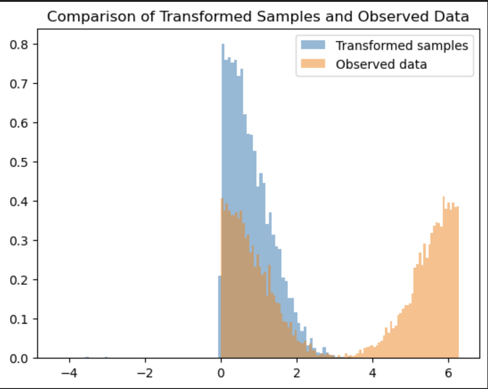
Could anyone recommend a practical transform that I could use to model this multimodal distribution? It consists of two peaks with a hump between them.