How to improve sampling in case of n_eff rather low?

Hi Numpyro fans,

I have a 21 parameters sampling to manage and I am using Numpyro NUTS with a model consisting of Uniform priors for same variables and Normal priors for the others, and finally the likelihood is a MultivariateNormal(signal, cov) distribution where cov is a constant covariance matrix 2250 x 2250. Now,

I use a simple running

nuts_kernel = numpyro.infer.NUTS(cond_model,
init_strategy=numpyro.infer.init_to_sample(),
max_tree_depth=5) # max_tree_depth=10

mcmc = numpyro.infer.MCMC(nuts_kernel,
num_warmup=1_000,
num_samples=8_000,
num_chains=1,
jit_model_args=True,
progress_bar=False)

The job summary indicates that r_hat is 1.00-1.01 while the n_eff for some variables are O(150) but some most are about 50 which is rather low effeiciency.

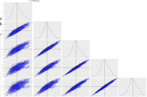
I have identified that 5 variables are highly correlated.
image

Do you have some advises to make the sampling more efficient? what about the mass matrix shaping for instance ?

I think you can try suggestions in the Bad posterior geometry and how to deal with it — NumPyro documentation tutorial.

Thanks @fehiepsi
o Considering for instance mass matrix structure do you think that using
dense_mass=[(“x1”,“x2”,“x3”,“x4”,“x5”)]
for the 5 correlated variables is a good starting point?
o Although using higher max_depth helps, above 5 is very demanding in my use-case.
o About SVI, does the same Numpyro model can be used ? (seems yes but I prefer to ask)

Yes to all. If you use SVI, it is good to start with autoguides like AutoNormal, which is ADVI in literatures.

1 Like

Hi @fehiepsi
Thanks for your clear advises. I just wanted

  1. if I have a

# gets some mock data
....
# compute Cov and Precision matrices : C & P
...
def model(data):
 # the priors numpyro.sample statement
....
 # compute signal 
...
 return numpyro.sample('signal', dist.MultivariateNormal(signal, 
                                                        precision_matrix=P,
                                                        covariance_matrix=C), obs=data) 

Then, I have defined

guide = autoguide.AutoNormal(model)
optimizer = numpyro.optim.Adam(step_size=0.05)
svi = SVI(observed_model, guide,optimizer,loss=Trace_ELBO())
svi_result = svi.run(jax.random.PRNGKey(0), 1000, data)

Notably I was asking myself:

  1. does the guide should not be attached to the model without the observations?
  2. in the context of NUTS, the initialisation can be init_strategy=numpyro.infer.init_to_sample(), here in the context of SVI how is performed the initialisation???
  3. I have run with the above code and got rather strange behavior: negative Trace_ELBO
    => may be Trace_ELBO or AutoNormal are not ad equa and I should use AutoMultivariateNormal but then with which loss?
  4. Is there a way to get the loss evolution plot to see if there is a convergence plateau?

After playing a bit


optimizer = numpyro.optim.Adam(step_size=0.005)
guide = autoguide.AutoMultivariateNormal(model, init_loc_fn=numpyro.infer.init_to_sample())
svi = SVI(model, guide,optimizer,loss=numpyro.infer.Trace_ELBO())
svi_result = svi.run(jax.random.PRNGKey(0), 10000, data)

I get

100%|█████████████████| 10000/10000 [1:17:00<00:00,  2.16it/s, init loss: 42777.1691, avg. loss [9501-10000]: -37425.6615]

but the if I use

predictive = Predictive(guide, params=svi_result.params, num_samples=5000)
samples = predictive(jax.random.PRNGKey(1), data)

the sampling looks strange (ie gaussian like although the distrib mean a far from the truth for all variables…)

Look like you got most issues resolved. The remaining one is

guide = autoguide.AutoNormal(observed_model)

(Otherwise the guide will think likelihood is a latent variable).

You can plot losses using svi_result.losses.

Heuu, considering your remark

guide = autoguide.AutoNormal(observed_model)

I do not understand may be you refer to a pervious version of this post that I have corrected: so does the following statements are correct considering the above structure of the model function? I had a look and try to follow the AutoDAIS example but lay I am wrong

guide = autoguide.AutoNormal(model)
or
guide = autoguide.AutoMultivariateNormal(model, init_loc_fn=numpyro.infer.init_to_sample())

By the way does it makes sense to get this ELBO loss behavior during Adam optim?
image

Yes, it makes sense (negative loss is sometimes fine if that’s your concern, you might want to enable x64 for better numerical calculations, especially those involve Cholesky like in MVN). I modified your code by changing model to observed model (in your early code version), if that’s your question. You can see some SVI examples from those tutorials SVI Part I: An Introduction to Stochastic Variational Inference in Pyro — Pyro Tutorials 1.8.4 documentation

Ok thanks @fehiepsi

I had read the nice Pyro doc you point, but what is very puzzling is this

Just like the model, the guide is encoded as a stochastic function guide() that contains 
pyro.sample and pyro.param statements. 

It does not contain observed data, since the guide needs to be a properly normalized distribution.

of course it is in the Pyro-framework, and Numpyro is a little different (?) but in the case of autoguide the “guide” code is automatically generated by looking at the model provided by the user (right?). And a long this line, the model has the likelihood statement with observed data, ie. something like

return numpyro.sample('y', dist.MultivariateNormal(cl, 
                                                        precision_matrix=P,
                                                        covariance_matrix=C),
                          obs=data)

So it is why the Pyro doc is quite confusing in the context of autoguide, no?

Does

from jax.config import config
config.update("jax_enable_x64", True)

enable also Numpyro x64 behavior?

I don’t quite understand what’s your question? Are those ? are questions or just to emphasize/double check? The guide should not contain observed site, as you quoted. I guess you wanted to mention some confusing point - could you elaborate that? (Your code follows best practices but I’m not sure what’s your concern)

Debugging point that to AutoGuide MultiVariateNormal output an non-definite positive covariance matrix : ie. scipy eigen decomposition shows negative eigen values. The point is that scipy.linalg.cholesky based on Lapack for instance does not raise error except when lower=True argument is explicitly set.

Interesting, does “covariance matrix” come from the MVN guide or from the model? If it comes from the guide, could you upload your svi_result or the guide’s covariance matrix somewhere so I can enhance the guide’s parameterization? (Unless model generates nan values, the guide covariance matrix should not be non-definite) If it comes from the model, you need to address that issue (in your code that calculates the covariance matrix of the likelihood).

Hi @fehiepsi
It is the guide_trace['auto_scale_tril']['value']matrix. If you wish I can sent to you the svi_result that I have hopefully saved :slight_smile:

Sure, I think we should address that numerical issue. Thanks!

Btw, could you try to add to this line

diag = jnp.clip(diag, a_min=jnp.finfo(diag.dtype).tiny)

to see if the problem goes away?

Hi @fehiepsi

How do think I can proceed to this line addition? as it is part of the Numpyro library, no?

I think you can uninstall the current version, then install a dev version with

git clone https://github.com/pyro-ppl/numpyro.git
cd numpyro
# install jax/jaxlib first for CUDA support
pip install -e .

then you can modify the source code in numpyro folder. That would behave like you install a release version - with an additional benefit that you can modify the source code. For developing/testing, we typically use the dev version, rather than the release versions on PyPI.

ha ! ok I will try asap and let you know. Thanks

Hi @fehiepsi
I have add the line as teh following lines in class SoftplusLowerCholeskyTransform(Transform)

        diag = softplus(x[..., -n:])
        diag = jnp.clip(diag, a_min=jnp.finfo(diag.dtype).tiny) ####JEC/DU
        return z + jnp.expand_dims(diag, axis=-1) * jnp.identity(n)

Remind that with the standard Numpyro version I got

scipy.linalg.eigvalsh(cov_mtx)
array([-0.07783337, -0.06924233, -0.03830554, -0.01789377, -0.0059395 ,
        0.00183724,  0.00523341,  0.01097751,  0.01314316,  0.01835902,
        0.02327265,  0.03061616,  0.03177506,  0.04952865,  0.05483383,
        0.05734573,  0.09309918,  0.12094973,  0.15347983,  0.15643385,
        0.26808384])

Now, with the new run may be the situation is going better but still the loss behaviour is the same and more importantly the cov matrix is still Non-DP, as there is still one negative eigen-value

scipy.linalg.eigvalsh(cov_mtx)
array([-0.04128681,  0.02607654,  0.03805184,  0.0445479 ,  0.05727365,
        0.06669969,  0.073379  ,  0.07424099,  0.07551433,  0.0794809 ,
        0.08118924,  0.08282787,  0.08391205,  0.08670352,  0.09583162,
        0.10654701,  0.11219324,  0.12001006,  0.12432292,  0.1331782 ,
        0.22785095])

@campagne Thanks for the data! It seems that by “covariance matrix”, you are talking about the scale_tril parameter, which is the cholesky of the covariance matrix. Using your notation, what you should check is:

scipy.linalg.eigvalsh(cov_mtx @ cov_mtx.T)