Hi there,
I have tried to get started with bayesian optimal experimental design. I have used the working memory example as initially, my setup can be made as a multilinear regression model. I am not super experienced with statistical models / probabilistic programming, so I am hoping one of you can look over the code and tell me if I have made some dumb mistakes. Lastly as you’ll see, i have a parameter constraint problem when I try to estimate marginal_eig.
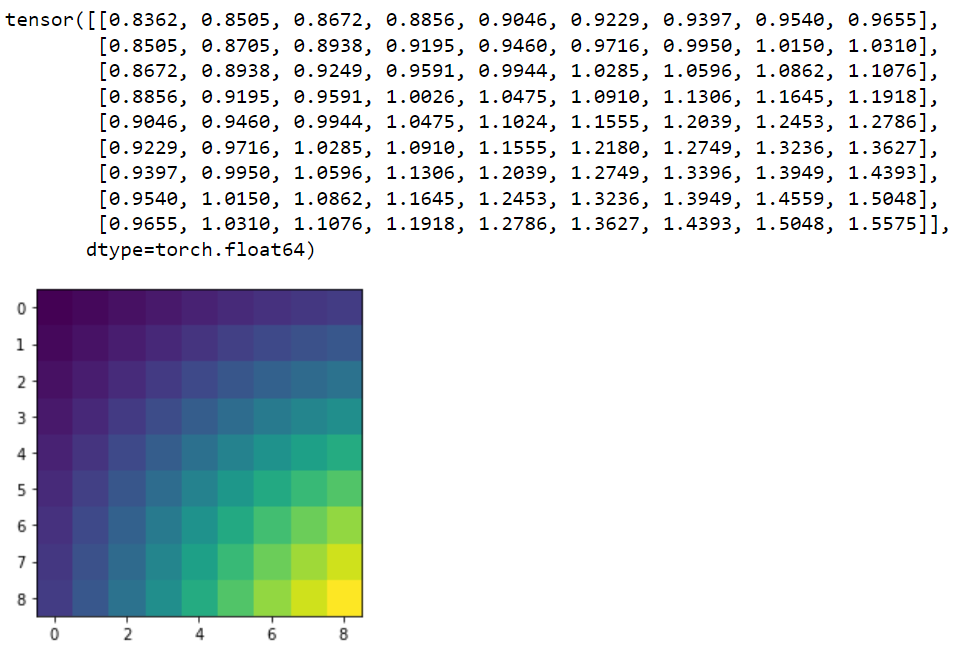
So far, I have been able to condition a model and it looks like productive results, so at least its not too terrible. I have made a simple 2d synthetic toy dataset as follows:
The practical idea for if/when this works, is to create a statistical experimental design in the design space, then compute an initial multilinear regression model the classical way, which serves as initial coefficients for the probabilistic model. Then do adaptive experiments using EIG from there.
import torch
import pyro
import pyro.distributions as dist
import matplotlib
import matplotlib.pyplot as plt
from torch.distributions.constraints import positive
from pyro.infer import SVI, Trace_ELBO
from pyro.optim import Adam
from pyro.contrib.oed.eig import marginal_eig
import torch.nn.functional as F
import numpy as np
from sklearn.metrics import mean_squared_error
from skimage.filters import gaussian
from sklearn.linear_model import LinearRegression
Initial design of the corners and centerpoint of the above dataset and an MLR model on that yielded some coefficients whichi is my starting point. The model is as follows:
c1_mean = torch.tensor(0.0026)
c1_sd = torch.tensor(c1_mean0.1)
c2_mean = torch.tensor(0.0189)
c2_sd = torch.tensor(c2_mean0.1)def model(l):
with pyro.plate_stack(“plate”, l.shape[:-1]):
coeff1 = pyro.sample(“coeff1”, dist.Normal(c1_mean, c1_sd))
coeff2 = pyro.sample(“coeff2”, dist.Normal(c2_mean, c2_sd))coeff1 = coeff1.unsqueeze(-1) coeff2 = coeff2.unsqueeze(-1) #levels of design level1,level2 = get_levels_eig(l) #MLR. I added a small bias to force non-zero values. seemed to solve one error pred = level1*coeff1+level2*coeff2+0.00001 y = pyro.sample("y", dist.Normal(pred,pred*0.1).to_event(1)) return y
The idea is to take in a design (value between 0 and 81). i call them well numbers in the code below because the actual experiments would run in a small plastic plate with wells in them (containing liquid). From this design, retrieve the actual levels of each variable (function for that is in the next code block below), calculate y by multiplying the levels of the variables with the coefficients. Without much knowledge, I suppose the coefficients and y would be normally distributed. As you can see I have initially set the standard deviations as 10% of the mean.
is there a better way to initialize the standard deviation?
Does the model look sane?
def get_levels(well_num):
factor1_levels = [0,20,40,60,80,100,120,140,160]
factor2_levels = [4,6,8,10,12,14,16,18,20]levels = [] for f1 in factor1_levels: for f2 in factor2_levels: levels.append([f1,f2]) level1 = torch.zeros_like(well_num) level2 = torch.zeros_like(well_num) if len(well_num.shape)==1: for w,well in enumerate(well_num): level1[w] = levels[int(well)][0] level2[w] = levels[int(well)][1] else: for s in range(well_num.shape[0]): for w in range(well_num.shape[1]): well_n = well_num[s,w,0] level1[s,w,0]=levels[int(well_n.item())][0] level2[s,w,0]=levels[int(well_n.item())][1] return level1,level2
A guide for SVI
def guide(l):
# The guide is initialised at the prior
c1_pmean = pyro.param(“c1_pmean”, c1_mean.clone(), constraint=positive)
c1_psd = pyro.param(“c1_psd”, c1_sd.clone(), constraint=positive)
c2_pmean = pyro.param(“c2_pmean”, c2_mean.clone(), constraint=positive)
c2_psd = pyro.param(“c2_psd”, c2_sd.clone(), constraint=positive)pyro.sample("coeff1", dist.Normal(c1_pmean, c1_psd)) pyro.sample("coeff2", dist.Normal(c2_pmean, c2_psd))
Here again I have initialized the standard deviation for the parameters as 10% of the mean and everything as normally distributed.
Conditioning a model with the initial design (corners and centerpoint) yields a much lower MSE of the MLR model on the full synthetic dataset. so it seems productive.
design = torch.tensor([0, 8, 65, 37, 80])
measured = torch.from_numpy(data_vector[design])conditioned_model = pyro.condition(model, {“y”: measured})
svi = SVI(conditioned_model,
guide,
Adam({“lr”: .001}),
loss=Trace_ELBO(),
num_samples=100)pyro.clear_param_store()
num_iters = 2000
for i in range(num_iters):
elbo = svi.step(design)
if i % 500 == 0:
print(“Neg ELBO:”, elbo)
Defining a marginal guide I was quite unsure how to do that. But taking the example from working memory, I stuck to the definition of the parameter as torch.zeros based on length of design and changed the “y” dist to be the same as within the model. Does this make sense?
def marginal_guide(design, observation_labels, target_labels):
# This shape allows us to learn a different parameter for each candidate design l
pred = pyro.param(“pred”, torch.ones(design.shape[-2:]), constraint=positive)
pyro.sample(“y”, dist.Normal(pred,pred*0.1).to_event(1))
I have estimated the marginal_eig with the code below:
#set coefficient means to initial MLR coefficients and SD to 10%
c1_mean = torch.tensor(0.0026)
c1_sd = torch.tensor(c1_mean0.1)
c2_mean = torch.tensor(0.0189)
c2_sd = torch.tensor(c2_mean0.1)#test all possible options
candidate_designs = torch.arange(0, 81, dtype=torch.float).unsqueeze(-1)pyro.clear_param_store()
num_steps, start_lr, end_lr = 1000, 0.1, 0.001
optimizer = pyro.optim.ExponentialLR({‘optimizer’: torch.optim.Adam,
‘optim_args’: {‘lr’: start_lr},
‘gamma’: (end_lr / start_lr) ** (1 / num_steps)})eig = marginal_eig(model,
candidate_designs, # design, or in this case, tensor of possible designs
“y”, # site label of observations, could be a list
[“coeff1”,“coeff2”], # site label of ‘targets’ (latent variables), could also be list
num_samples=100, # number of samples to draw per step in the expectation
num_steps=num_steps, # number of gradient steps
guide=marginal_guide, # guide q(y)
optim=optimizer, # optimizer with learning rate decay
final_num_samples=10000 # at the last step, we draw more samples
# for a more accurate EIG estimate
)
The EIGs are as follows:
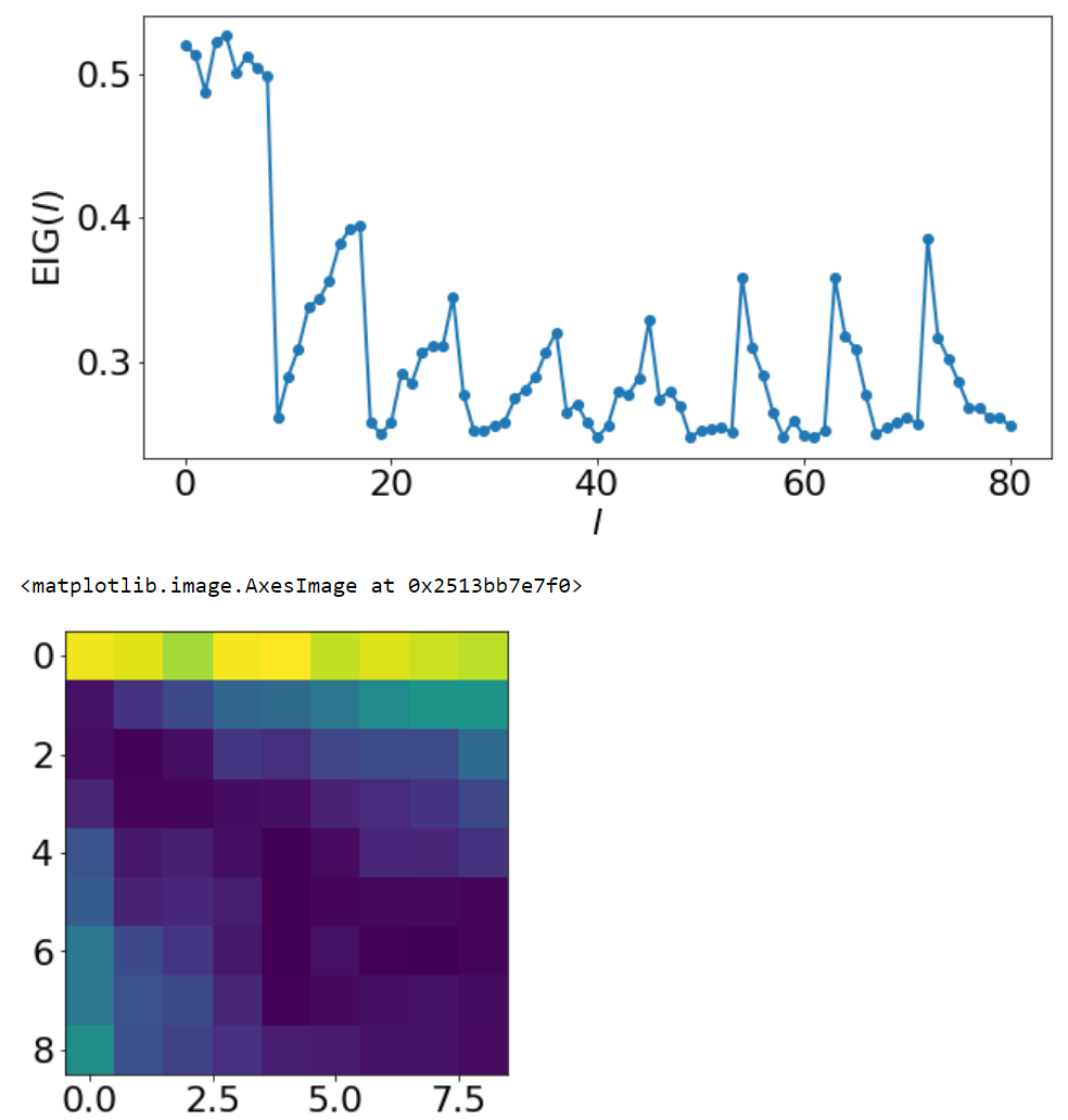
Attached them here in case it indicates a suboptimal part somewhere in my code… I feel like its promising that most of the high EIGs are distributed out in the space, but the initial 9 high values seem abnormal?