I’m trying to implement one of the examples from Chapter 6 of [1] but I can’t get the same result. The model is a simple Capture-Recapture model with 3 observation periods and constant probabilities of recapture. The object of interest is N, the true population size of the species being studied, and the model uses data augmentation to estimate it. The augmented data is yaug, which is built by appending rows of zeros to the observed capture histories binary array yobs, which has dimension C x T where C is the total individuals captured and T is the number of observation periods. Then a discrete latent variable z is used in the model to account for weather a specimen is ever captured.
This is the R code of their implementation in WinBugs:
# Augment data set by 150 potential individuals nz <- 150 yaug <- rbind(data$yobs, array(0, dim = c(nz, data$T)))

# Specify model in BUGS language sink("model.txt") cat(" model {

# Priors
omega ~ dunif(0, 1)
p ~ dunif(0, 1)

# Likelihood
for (i in 1:M){
   z[i] ~ dbern(omega)
   for (j in 1:T){
      # Inclusion indicators
      yaug[i,j] ~ dbern(p.eff[i,j])
      p.eff[i,j] <- z[i] * p # Can only be detected if z=1
      } #j
   } #i

# Derived quantities
N <- sum(z[])
} ",fill = TRUE)
sink()
And this is my implementation in numpyro:
def model_6_2(nz=150, yobs=None):
    N, T = yobs.shape if yobs is not None else (100, 3)
    M = N + nz    # nz is the number of individuals added through data-augmenation
    # Augment data by adding rows of zeros:
    yaug = jnp.vstack([yobs, jnp.zeros(shape=(nz, T))]) if yobs is not None else None
    omega = npr.sample("omega", dist.Beta(2, 2))
    p = npr.sample("p", dist.Beta(2, 2))
    with npr.plate("Animals", M, dim=-2):
        z = npr.sample("z", dist.Bernoulli(probs=omega),
            infer={"enumerate": "parallel"}) # Inclusion indicator.
        with npr.plate("Time", T, dim=-1):
            npr.sample("y_aug", dist.Bernoulli(z * p), obs=yaug)

    # Two ways get estimated population size (give ~ same result):
    npr.deterministic("N_est1", M * omega)
    npr.deterministic("N_est1", jnp.sum(z))
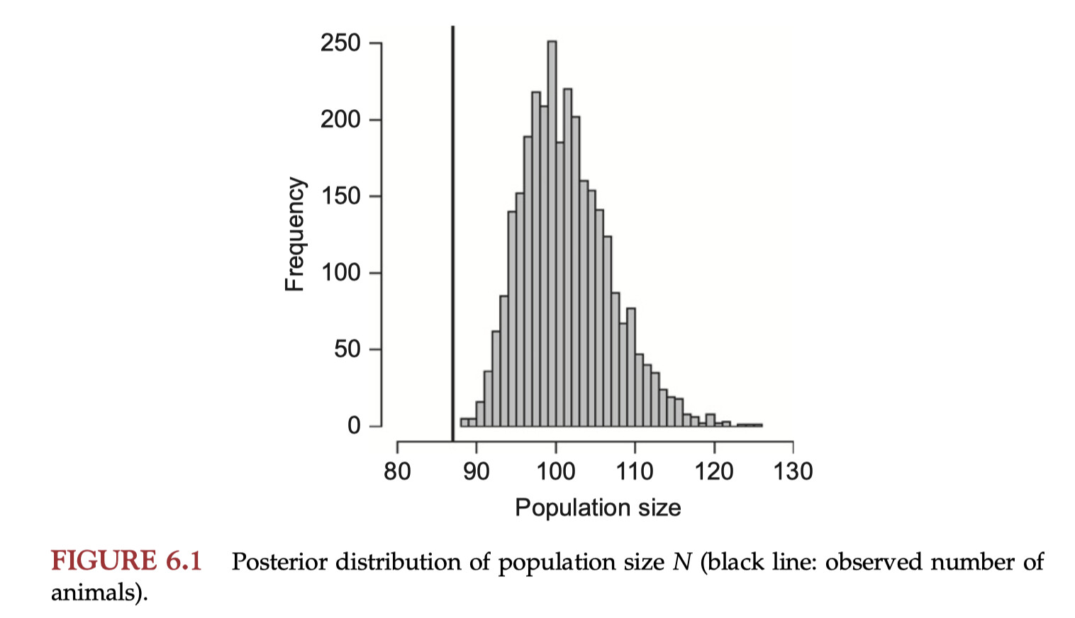
In the book they report the following posterior for the true population size, N:
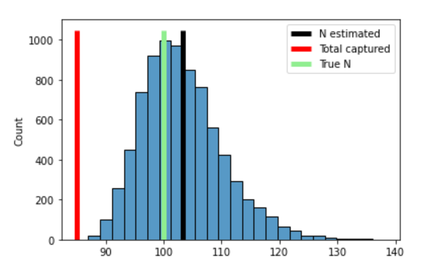
while I get (see section below for the code that made this plot):
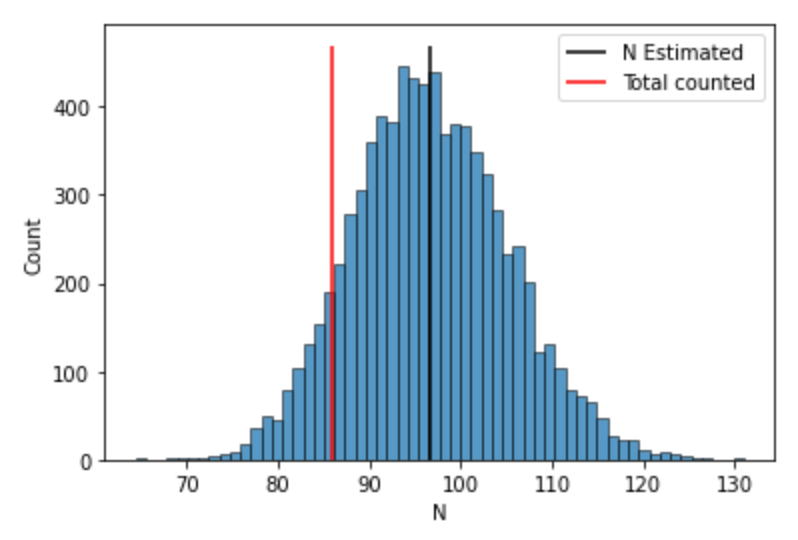
The posterior mean is correct, but my distribution for N is too wide.
Simulating the data and running the code
I simulate the data using
def data_fn(N=100, p=0.5, T=3):
    yfull = np.random.binomial(n=1, p=p, size=(N, T))
    ever_detected = np.max(yfull, axis=1) # Binary, 1 if animal was ever catched.
    C = np.sum(ever_detected) # Total number of animals catched.
    yobs = yfull[ever_detected==1]
    print(f"{C} out of {N} animals present where detected.\n")
    return dict(N=N, p=p, C=C, T=T, yfull=yfull, yobs=yobs)

data = data_fn()
And run the model using
import numpyro as npr
import numpyro.distributions as dist
from numpyro.infer import Predictive, NUTS, HMC, MCMC
import jax.numpy as jnp
import jax.random as random
import jax.lax as lax
import numpy as np

key = random.PRNGKey(235)

def run_inference(model, rng_key, args, **kwargs):
    if args.algo == "NUTS":
        kernel = NUTS(model)
    elif args.algo == "HMC":
        kernel = HMC(model)
    mcmc = MCMC(
        kernel,
        num_warmup=args.num_warmup,
        num_samples=args.num_samples,
        num_chains=args.num_chains,
    )
    mcmc.run(rng_key, **kwargs)
    mcmc.print_summary()
    return mcmc.get_samples()

class Args:
    pass

args = Args()
args.algo = "NUTS"
args.num_warmup = 500
args.num_samples = 2000
args.num_chains = 4

key, subkey = random.split(key)
posterior = run_inference(model_6_2, subkey, args, **{"yobs": data["yobs"]})

# Plot histogram:
sns.histplot(posterior["N_est1"])
ymax = plt.gca().get_ylim()[1]
plt.vlines(posterior["N_est1"].mean(), 0, ymax, color="k", label="N Estimated")
plt.vlines(data["C"].mean(), 0, ymax, color="r", label="Total counted")
plt.xlabel("N")
plt.legend()
[1] Kéry, Marc, and Michael Schaub. Bayesian population analysis using WinBUGS: a hierarchical perspective . Academic Press, 2011.