Get site name after NeuTraReparam.reparam

Hello,
How to get the site names after

from numpyro.infer.reparam import NeuTraReparam
from numpyro.infer import MCMC, NUTS, init_to_sample

neutra = NeuTraReparam(guide, svi.get_params(carry[1])) 
neutra_model = neutra.reparam(model_spl)

Notice that neutra is defined after a SVI processing on model_spl.

I would like to get the list of sites of neutra_model for instance to tune the dense_mass parameter of

nuts_kernel = NUTS(neutra_model,
                  init_strategy=numpyro.infer.init_to_median(),
                   dense_mass=True,
                   max_tree_depth=5)

Thanks

Hi @campagne, you can use trace handler to get site names of numpyro models, including the neutra model.

Well,
if I manage to trace the original model (model_spl), here is the error for the netra_model:

tr = numpyro.handlers.trace(seed(neutra_model, jax.random.PRNGKey(0)))
tr.get_trace()

I get this trace back

AssertionError Traceback (most recent call last)
in
----> 1 tr.get_trace()

/numpyro/handlers.py in get_trace(self, *args, **kwargs)
163 :return: OrderedDict containing the execution trace.
164 “”"
→ 165 self(*args, **kwargs)
166 return self.trace
167

/numpyro/primitives.py in call(self, *args, **kwargs)
85 return self
86 with self:
—> 87 return self.fn(*args, **kwargs)
88
89

/numpyro/primitives.py in call(self, *args, **kwargs)
85 return self
86 with self:
—> 87 return self.fn(*args, **kwargs)
88
89

/numpyro/primitives.py in call(self, *args, **kwargs)
85 return self
86 with self:
—> 87 return self.fn(*args, **kwargs)
88
89

in model_spl(cl_obs)

numpyro/primitives.py in sample(name, fn, obs, rng_key, sample_shape, infer, obs_mask)
198
199 # …and use apply_stack to send it to the Messengers
→ 200 msg = apply_stack(initial_msg)
201 return msg[“value”]
202

/numpyro/primitives.py in apply_stack(msg)
22 pointer = 0
23 for pointer, handler in enumerate(reversed(_PYRO_STACK)):
—> 24 handler.process_message(msg)
25 # When a Messenger sets the “stop” field of a message,
26 # it prevents any Messengers above it on the stack from being applied.

numpyro/handlers.py in process_message(self, msg)
552 return
553
→ 554 new_fn, value = reparam(msg[“name”], msg[“fn”], msg[“value”])
555
556 if value is not None:

/numpyro/infer/reparam.py in call(self, name, fn, obs)
253 if not self._x_unconstrained: # On first sample site.
254 # Sample a shared latent.
→ 255 z_unconstrained = numpyro.sample(
256 “{}_shared_latent”.format(self.guide.prefix),
257 self.guide.get_base_dist().mask(False),

/numpyro/primitives.py in sample(name, fn, obs, rng_key, sample_shape, infer, obs_mask)
198
199 # …and use apply_stack to send it to the Messengers
→ 200 msg = apply_stack(initial_msg)
201 return msg[“value”]
202

/numpyro/primitives.py in apply_stack(msg)
39 # via the pointer variable from the process_message loop
40 for handler in _PYRO_STACK[-pointer - 1 :]:
—> 41 handler.postprocess_message(msg)
42 return msg
43

/numpyro/handlers.py in postprocess_message(self, msg)
148 # which has no name
149 return
→ 150 assert not (
151 msg[“type”] == “sample” and msg[“name”] in self.trace
152 ), “all sites must have unique names but got {} duplicated”.format(

AssertionError: all sites must have unique names but got auto_shared_latent duplicated

Seems like something is wrong. Could you make a reproducible code? (FYI, your code works for neutra example with numpyro master github branch).

Hi @fehiepsi here is some material for debugging.

I’m using

numpyro                   0.8.0              pyhd8ed1ab_0    conda-forge

Now here is a snippet that reproduces the problem

import numpy as np
import jax

import jax.numpy as jnp
import numpyro
import numpyro.distributions as dist
import numpyro.infer.autoguide as autoguide
from numpyro.infer import Predictive, SVI, Trace_ELBO,  TraceMeanField_ELBO
from numpyro.optim import Adam
from numpyro.infer.reparam import NeuTraReparam
from numpyro.handlers import seed, trace, condition

#Generate mock data
param_true = np.array([1.0, 0.0, 0.2, 0.5, 1.5])
sample_size = 1_000
sigma_e = param_true[4]          # true value of parameter error sigma
random_num_generator = np.random.RandomState(0)
xi = 5*random_num_generator.rand(sample_size)-2.5
e = random_num_generator.normal(0, sigma_e, sample_size)
yi = param_true[0] + param_true[1] * xi + param_true[2] * xi**2 + param_true[3] *xi**3# +  e  

# Simple model
def my_model(Xspls,Yspls=None):
    a0 = numpyro.sample('a0', dist.Normal(0.,10.))
    a1 = numpyro.sample('a1', dist.Normal(0.,10.))
    a2 = numpyro.sample('a2', dist.Normal(0.,10.))
    a3 = numpyro.sample('a3', dist.Normal(0.,10.))

    mu = a0 + a1*Xspls + a2*Xspls**2 + a3*Xspls**3

    return numpyro.sample('obs', dist.Normal(mu, sigma_e), obs=Yspls)

#Simple SVI
guide = autoguide.AutoMultivariateNormal(my_model, init_loc_fn=numpyro.infer.init_to_sample())
optimizer = numpyro.optim.Adam(step_size=5e-3)
svi = SVI(my_model, guide,optimizer,loss=Trace_ELBO())
svi_result = svi.run(jax.random.PRNGKey(0), 10000, Xspls=xi, Yspls=yi)

#Neutra-reparametrisation
neutra = NeuTraReparam(guide, svi_result.params)
neutra_model = neutra.reparam(my_model)

#Tracing the original model (It is working)
tr = numpyro.handlers.trace(seed(my_model, jax.random.PRNGKey(0)))
tr.get_trace(Xspls=xi)

#Tracing the neutra_model (ERROR)
tr = numpyro.handlers.trace(seed(neutra_model, jax.random.PRNGKey(0)))
tr.get_trace(Xspls=xi)

The end of the tracing gives

AssertionError: all sites must have unique names but got `auto_shared_latent` duplicated

It seems that the missing data yi is causing NeuTra to reparam the likelihood. You can specify yi in the get_trace method to resolve the issue. But the error message is misleading. Could you add a github issue for a better error message?

Ha. ok so for the snippet

tr.get_trace(Xspls=xi, Yspls=yi)

works fine, and for my larger pb also it is ok if I provides all args of the original model.

But I have one more question, in the trace I have the following structure

`auto_shared_latent`
{'type': 'sample',
               'name': 'auto_shared_latent',
               'fn': <numpyro.distributions.distribution.MaskedDistribution at 0x2ba4e7412df0>,
               'args': (),
               'kwargs': {'rng_key': array([2718843009, 1272950319], dtype=uint32),
                'sample_shape': ()},
               'value': DeviceArray([ 1.00499645, -1.17144072,  1.36345258,  0.20145079,
                             0.10308774,  0.94062874, -0.09197039,  0.78612585,
                            -0.23571828,  0.34550364, -0.66854574,  1.23069877,
                             0.1425439 , -1.18842738,  0.59869803,  0.49498235,
                            -0.15488275, -0.22944503, -0.68945286, -1.15955295,
                             1.76636159], dtype=float64),
               'scale': None,
               'is_observed': False,
               'intermediates': [],
               'cond_indep_stack': [],
               'infer': {}}),

Then a list of <var> from my original model and <var>_log_prob

('_<var>_log_prob',
              {'type': 'sample',
               'name': '_<var>_b_log_prob',
               'fn': <numpyro.distributions.distribution.Unit at 0x2bad901798b0>,
               'args': (),
               'kwargs': {'rng_key': None, 'sample_shape': ()},
               'value': DeviceArray([], dtype=float64),
               'scale': None,
               'is_observed': True,
               'intermediates': [],
               'cond_indep_stack': [],
               'infer': {}}),
             ('<var>',
              {'type': 'deterministic',
               'name': '<var>',
               'value': DeviceArray(0.04561563, dtype=float64)}),

.....
Then the observations

('cl',
              {'type': 'sample',
               'name': 'cl',
               'fn': <numpyro.distributions.continuous.MultivariateNormal at 0x2bad92c2c4c0>,
               'args': (),
               'kwargs': {'rng_key': None, 'sample_shape': ()},
               'value': DeviceArray([8.99140109e-09, 8.45213802e-09, 7.86886926e-09, ...,
                            1.21885897e-06, 1.07332405e-06, 9.49056238e-07],            dtype=float64),
               'scale': None,
               'is_observed': True,
               'intermediates': [],
               'cond_indep_stack': [],
               'infer': {}})])

How I can modifiy the dense mass matrix structure in the following code using the neutra_model?

nuts_kernel = NUTS(neutra_model,
                  init_strategy=numpyro.infer.init_to_feasible(), #was median
                   dense_mass= ????
                   max_tree_depth=5)

Thanks

I think you can set dense_mass=True there. There is only 1 latent variable in your model: auto_shared_latent. The other variables are observed (including log prob factors).

Oups! Then I am not sure of what I was expecting :frowning:

I start with a model_spl with 21 priors variables and likelihood with observations

Then I use SVI to approximate the posterior with AutoMultivariateNormal

guide = autoguide.AutoMultivariateNormal(model_spl,                                      init_loc_fn=numpyro.infer.init_to_value(values=true_param))                                         

Then NeutraReparam

neutra = NeuTraReparam(guide, svi.get_params(carry[1])) #  svi_result.params
neutra_model = neutra.reparam(model_spl)

to perform NUTS

I was expecting to get SVI model with 21 parameters and an approximation of the MultivariateNormal of the model_spl posterior ???

When you use NeuTra, the latent variable is auto_shared_latent. Other latent variables in your original model are determistic transformed (decided by guide optimized parameters) from this auto_shared_latent variable. If you have 21 scalar variables in your model, the auto shared latent will have size 21.

Hello @fehiepsi

Let me try with few equations/notations to be more explicit

In this first slide, I try to summarize the SVI challenge to approximate the posterior distribution of latent variables (vector z of dim N=21) with a q-distribiution depending on lambda parameters. Here I choose q-dist as a multivariate normal, with lambda the collection of mean (mu) and square root of a cov matrix (L)) parameters. So, mu is a vector of dimension N and L is a lower-triangle of dim N(N+1)/2. So N+N(N+1)/2 parameters for lambda.

In this second slide, I try to make the Neutra Reparam explicit in the case of q-dist as a multivariate normal. (nb. May be I have omitted over reparametrisation from original priors eg. Uniform-dist which may take place before Neutra one.But let us omit this technicality by using original gaussian priors for instance.)

Using this reparametrisation I can draw \xi samples from the modified q(z;\lambda^\ast) distrib, to initiate NUTS sampling on p(\xi, D). Then, using the inverse transformation I get Markov chain on the original z-latent variables.

image

So far so good. But coming back to \lambda I would expect N+N(N+1)/2 parameters to define the SVI (Multi-variate Normal distribution, N for the mean mu and N(N+1)/2 to get the covariance sym def. pos. matrix. It is why I am surprise by

('auto_shared_latent',
              {'type': 'sample',
               'name': 'auto_shared_latent',
               'fn': <numpyro.distributions.distribution.MaskedDistribution at 0x2ba4e7412df0>,
               'args': (),
               'kwargs': {'rng_key': array([2718843009, 1272950319], dtype=uint32),
                'sample_shape': ()},
               'value': DeviceArray([ 1.00499645, -1.17144072,  1.36345258,  0.20145079,
                             0.10308774,  0.94062874, -0.09197039,  0.78612585,
                            -0.23571828,  0.34550364, -0.66854574,  1.23069877,
                             0.1425439 , -1.18842738,  0.59869803,  0.49498235,
                            -0.15488275, -0.22944503, -0.68945286, -1.15955295,
                             1.76636159], dtype=float64),
               'scale': None,
               'is_observed': False,
               'intermediates': [],
               'cond_indep_stack': [],
               'infer': {}}),

In the ‘value’ of size N=21, I may guess that this is the mu-values, but what about the Cov matrix elements?

Using MVN guide, there are 2 params named loc and scale_tril. These params creates a bijective transform from auto_shared_latent to the (unconstrained+flatten+concatenate) latent variables in your model. I’m not sure how to put priors to those loc and scale parameters and perform MCMC to infer them. I guess one way is to write a new model with latent variables loc and scale, then specify it in the params input of NeuTra (rather than using svi.get_params). It might be buggy - I haven’t tried it in the past.

Well it would be nice to elaborate a snippet that I can try. Thanks

Sure, just heuristic,

def model(data):
    loc = numpyro.sample("loc", Normal(...))
    corr_cholesky = numpyro.sample("corr_cholesky", LKJCholesky(...))
    scale = numpyro.sample("scale", Exponential(...))
    scale_tril = corr_cholesky * scale[..., None]
    # check svi_result.params or svi.get_params(state) for correct keys
    params = {"auto_loc": loc, "auto_scale_tril": scale_tril}
    neutra = NeuTraReparam(guide, params)
    neutra_model = neutra.reparam(model_spl)
    return neutra_model(data)

Thanks @fehiepsi
Currently I cannot test your nice idea due to maintenance of the GPU cluster.
But, can you elaborate a little bit more what you mean as “…” in Normal/LKJCholesky/scale?

That code is user-defined priors for loc and scale_tril. You can use other priors for loc, e.g. Cauchy(0, 1) or Cauchy(0, 10). For scale tril, I used LKJ prior but you can use other priors like Wishart (not available in numpyro but available in tfp).

Hello @fehiepsi
I still do not have access to my GPU cluster, but I have set up a smaller use-case that we can dig a little bit more.

import numpy as np
import jax
import jax.numpy as jnp
from jax.config import config
config.update("jax_enable_x64", True)


import numpyro
import numpyro.distributions as dist
import numpyro.infer.autoguide as autoguide
from numpyro.infer import Predictive, SVI, Trace_ELBO,  TraceMeanField_ELBO
from numpyro.optim import Adam
from numpyro.infer.reparam import NeuTraReparam
from numpyro.handlers import seed, trace, condition
from numpyro.infer import MCMC, NUTS, init_to_sample
mpl.rc('image', cmap='jet')
mpl.rcParams['font.size'] = 18
mpl.rcParams["font.family"] = "Times New Roman"


import corner

import matplotlib as mpl
import matplotlib.pyplot as plt

#For contour ploting
#-----------------------
def plot_diagnostics(samples, param_true, samples_b=None, labels=None):
    mpl.rcParams['font.size'] = 12
    #DF ndim = len(samples.keys())
    ndim = samples.shape[1]
    # This is the empirical mean of the sample:
    ##DF value2 = np.mean(np.array(list(samples.values())),axis=1)
    value2 = np.mean(samples,axis=0)
    #True
    value1 = param_true

    # Make the base corner plot
    # 68% et 95% quantiles 1D et levels in 2D
    figure = corner.corner(samples,labels=labels,quantiles=(0.025, 0.158655, 0.841345, 0.975), levels=(0.68,0.95), 
                        show_titles=True, title_kwargs={"fontsize": 14}, 
                        truths=param_true, truth_color='g', color='b'
                        );
    if samples_b is not None:
        corner.corner(samples_b,labels=labels,quantiles=(0.025, 0.158655, 0.841345, 0.975), levels=(0.68,0.95), 
                        show_titles=True, title_kwargs={"fontsize": 14}, 
                        truths=param_true, truth_color='g', color='purple', fig=figure
                        );
    # Extract the axes
    axes = np.array(figure.axes).reshape((ndim, ndim))

    # Loop over the diagonal
    for i in range(ndim):
        ax = axes[i, i]
        ax.axvline(value2[i], color="r")
    
    # Loop over the histograms
    for idy in range(ndim):
        for idx in range(idy):
            ax = axes[idy, idx]
            ax.axvline(value2[idx], color="r")
            ax.axhline(value2[idy], color="r")
            ax.plot(value2[idx], value2[idy], "sr")

    return figure
####
# Mock data
####
param_true = np.array([1.0, 0.0, 0.2, 0.5, 1.5])
sample_size = 5_000
sigma_e = param_true[4]          # true value of parameter error sigma
random_num_generator = np.random.RandomState(0)
xi = 5*random_num_generator.rand(sample_size)-2.5
e = random_num_generator.normal(0, sigma_e, sample_size)
#e = np.zeros(sample_size)
yi = param_true[0] + param_true[1] * xi + param_true[2] * xi**2 + param_true[3] *xi**3# +  e  
plt.hist2d(xi, yi, bins=50);

###
# Simple Numpyro model
###
def my_model(Xspls,Yspls=None):
    a0 = numpyro.sample('a0', dist.Normal(0.,10.))
    a1 = numpyro.sample('a1', dist.Normal(0.,10.))
    a2 = numpyro.sample('a2', dist.Normal(0.,10.))
    a3 = numpyro.sample('a3', dist.Normal(0.,10.))

    mu = a0 + a1*Xspls + a2*Xspls**2 + a3*Xspls**3

    return numpyro.sample('obs', dist.Normal(mu, sigma_e), obs=Yspls)

### 
# Use NUTS sampling to get a reference
###
# Start from this source of randomness. We will split keys for subsequent operations.
rng_key = jax.random.PRNGKey(0)
_, rng_key, rng_key1, rng_key2 = jax.random.split(rng_key, 4)


# Run NUTS.
kernel = NUTS(my_model, init_strategy=numpyro.infer.init_to_median())
num_samples = 10_000
n_chains = 1
mcmc = MCMC(kernel, num_warmup=1_000, num_samples=num_samples,  
            num_chains=n_chains,progress_bar=True)
mcmc.run(rng_key, Xspls=xi, Yspls=yi)
mcmc.print_summary()
samples_nuts = mcmc.get_samples()
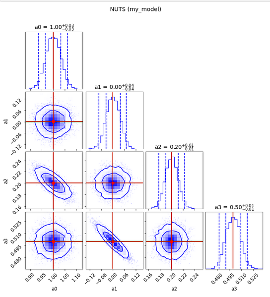
The result looks ok


                mean       std    median      5.0%     95.0%     n_eff     r_hat
        a0      1.00      0.03      1.00      0.95      1.05   4244.95      1.00
        a1      0.00      0.04      0.00     -0.06      0.06   5130.94      1.00
        a2      0.20      0.01      0.20      0.18      0.22   4405.43      1.00
        a3      0.50      0.01      0.50      0.48      0.51   5174.54      1.00

Number of divergences: 0

Do the contour plots

labels = [*samples_nuts]
values = np.array(list(samples_nuts.values())).T
fig = plot_diagnostics(values, param_true[:-1], labels=labels)
fig.suptitle("NUTS (my_model)",y=1.05);

Now perform a SVI with MVN guide

guide = autoguide.AutoMultivariateNormal(my_model, init_loc_fn=numpyro.infer.init_to_sample())
optimizer = numpyro.optim.Adam(step_size=5e-3)
svi = SVI(my_model, guide,optimizer,loss=Trace_ELBO())
svi_result = svi.run(jax.random.PRNGKey(0), 10000, Xspls=xi, Yspls=yi)

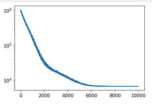
The loss decreases rather well

plt.plot(svi_result.losses)
plt.yscale('log')

image

Now perform the sampling of the optimised guide

samples_svi = guide.sample_posterior(jax.random.PRNGKey(1), svi_result.params, sample_shape=(5000,))

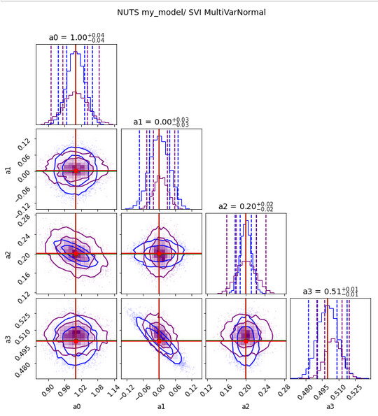
As you see below here is the comparison of the two set of contour plots

labels = [*samples_nuts]
values1 = np.array(list(samples_nuts.values())).T
values2 = np.array(list(samples_svi.values())).T
fig = plot_diagnostics(values1, param_true[:-1], samples_b=values2, labels=labels)
fig.suptitle("NUTS my_model/ SVI MultiVarNormal",y=1.05);

The blue contours are those of NUTS(my_model) and the others from the SVI optimized model

Now the Stnadard NeutraParam would be

from numpyro.infer.reparam import NeuTraReparam
neutra = NeuTraReparam(guide, svi_result.params)
neutra_model = neutra.reparam(my_model)

And one can perform a NUTS sampling based on this neutra_model as

# NUTS
####
nuts_kernel = NUTS(neutra_model)
mcmc_neutra = MCMC(nuts_kernel, num_warmup=1_000, num_samples=num_samples,  
            num_chains=n_chains,progress_bar=True)
mcmc_neutra.run(rng_key, Xspls=xi, Yspls=yi)
mcmc_neutra.print_summary()
#### 
#Get the MCMC  chain with the original latent variables
zs = mcmc_neutra.get_samples()["auto_shared_latent"]
samples_nuts_neutra = neutra.transform_sample(zs)

#Compare the contours
labels = [*samples_nuts]
values1 = np.array(list(samples_nuts.values())).T
values2 = np.array(list(samples_nuts_neutra.values())).T
fig = plot_diagnostics(values1, param_true[:-1], samples_b=values2, labels=labels)
fig.suptitle("NUTS my_model/ NUTS neutra MVN",y=1.05);

And one would be happy.

Well so far so good in the context of this simple exercice everything is rather ok. But already one can question the SVI optimized solution has the sampling of this solution leads to contour plots that barely fit the true solution. Notably we do not get as correlated features than one expects. So, for my more complex example, the SVI optimized solution looks very much as Normal Independent Gaussian priors. So, it is why we engaged the discussion on a new modelling.

I have not yet manage to get it right, and I need a little help. Looking at svi_results yields

SVIRunResult(params={'auto_loc': DeviceArray([0.99782024, 0.00510312, 0.20099757, 0.50513794], dtype=float64), 'auto_scale_tril': DeviceArray([[ 4.38094511e-02,  0.00000000e+00,  0.00000000e+00,
               0.00000000e+00],
             [ 3.83301696e-04,  2.65209844e-02,  0.00000000e+00,
               0.00000000e+00],
             [-8.11400370e-03, -1.22554246e-05,  1.90036797e-02,
               0.00000000e+00],
             [-4.52685904e-05, -4.21003102e-03,  6.09038196e-05,
               6.50602519e-03]], dtype=float64)}, state=SVIState(optim_state=(DeviceArray(10000, dtype=int64, weak_type=True), OptimizerState(packed_state=([DeviceArray([0.99782024, 0.00510312, 0.20099757, 0.50513794], dtype=float64), DeviceArray([ 16.40012248, -15.07899987,  39.20599832, -20.59373367], dtype=float64), DeviceArray([ 254334.14146581,   49334.38058495, 1307344.81640189,
              893760.92674789], dtype=float64)], [DeviceArray([ 1.44527703e-02, -4.26970136e-01, -6.44897449e-04,
             -6.95794883e-03, -6.47097252e-01,  9.36114107e-03,
             -3.10592101e+00, -3.61652920e+00, -3.95360576e+00,
             -5.03177180e+00], dtype=float64), DeviceArray([-0.6765813 , -1.07499804,  1.19968273, -0.60765637,
              0.50645236,  0.15576062,  0.20232971,  0.29539797,
              6.6081198 ,  2.87223864], dtype=float64), DeviceArray([  207.87352414, 12813.09351795, 13165.76001714,
              2787.26121383,  2849.72120231,  3101.19997409,
              2239.0793659 ,   201.43236727, 11896.08727525,
              2447.8603139 ], dtype=float64)]), tree_def=PyTreeDef({'auto_loc': *, 'auto_scale_tril': *}), subtree_defs=(PyTreeDef((*, *, *)), PyTreeDef((*, *, *))))), mutable_state=None, rng_key=DeviceArray([1267660082, 1240493033], dtype=uint32)), losses=DeviceArray([1017751.28605802,  988035.41332936, 1001172.51960345, ...,
                6660.3973429 ,    6648.90343705,    6646.57863752],            dtype=float64))

How how I can complete this new model and use it concretly with the material of my simple example?

def new_model(data):
    loc = numpyro.sample("loc", dist.Cauchy(0.,10.))
    concentration = jnp.ones(1)
    d = svi_result.params['auto_scale_tril'].shape[0]
    corr_cholesky = numpyro.sample("corr_cholesky", dist.LKJCholesky(d,concentration))
    scale = numpyro.sample("scale", Exponential(...))
    scale_tril = corr_cholesky * scale[..., None]
    # check svi_result.params or svi.get_params(state) for correct keys
    params = {"auto_loc": loc, "auto_scale_tril": scale_tril}
    neutra = NeuTraReparam(guide, params)
    neutra_model = neutra.reparam(my_model)
    return neutra_model(data)

I guess you can use Exponential(rate) prior for scale_tril, where rate is inverse of square root of the diagonal part of (auto_scale_tril @ auto_scale_tril.T). And for loc prior, you can use Normal(auto_loc, 1) I guess. I.e. I am setting priors based on my prior knowledge from svi results.