I am working on a modification of this for my use case.
http://pyro.ai/examples/forecasting_iii.html
My use case is that I have multiple traces (call them “regions”) with similar seasonal and trend models (but region-specific parameters) plus observation noise. So, this tutorial looks appropriate.
My time-varying covariate is an event trace indicating whether or not the system was exposed to an exogenous factor (regressor weight is constant but event data changes). I constructed this as a covariate tensor with the same dimensions of the data (observable) with ones indicating when the event occurs for each region at each time point.
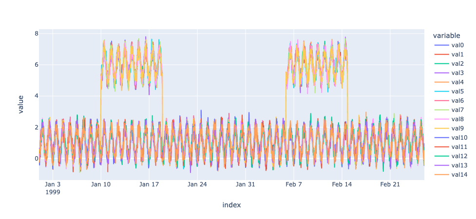
I modeled the effect of the exposure as a shift in baseline (though later I may want a linear multiplicative model on exposure-dose). The data is the sum of seasonal, exposure, and an OU process noise. It looks like this (colors are regions). I made two exposure periods for some regions for training and testing (split the data between the exposures). The data looks like this (and covariate tensor is similar but square-waves).
With trial and error, I modified the tutorial code Model as this:
class Model1(ForecastingModel):
    def model(self, zero_data, covariates):
        duration, data_dim = zero_data.shape
        # print(data_dim)
        feature = covariates
        # print(feature)
        exposure = pyro.sample("exposure", dist.Normal(0, 1))
        regressor = (exposure * feature).T
        # print(torch.max(regressor,dim=0))
        # Let's model each time series as a Levy stable process, and share process parameters
        # across time series. To do that in Pyro, we'll declare the shared random variables
        # outside of the "origin" plate:
        drift_stability = pyro.sample("drift_stability", dist.Uniform(1, 2))
        drift_scale = pyro.sample("drift_scale", dist.LogNormal(-20, 5))
        with pyro.plate("origin", data_dim, dim=-2):
            # Now inside of the origin plate we sample drift and seasonal components.
            # All the time series inside the "origin" plate are independent,
            # given the drift parameters above.
            with self.time_plate:
                # We combine two different reparameterizers: the inner SymmetricStableReparam
                # is needed for the Stable site, and the outer LocScaleReparam is optional but
                # appears to improve inference.
                with poutine.reparam(config={"drift": LocScaleReparam()}):
                    with poutine.reparam(config={"drift": SymmetricStableReparam()}):
                        drift = pyro.sample("drift",
                                            dist.Stable(drift_stability, 0, drift_scale))

            with pyro.plate("hour_of_week", 24 , dim=-1):
                seasonal = pyro.sample("seasonal", dist.Normal(0, 5))

        # Now outside of the time plate we can perform time-dependent operations like
        # integrating over time. This allows us to create a motion with slow drift.

        seasonal = periodic_repeat(seasonal, duration, dim=-1)
        motion = drift.cumsum(dim=-1)  # A Levy stable motion to model shocks.

        # print(f'regressor size = {regressor.size()}')
        # print(f'motion size = {motion.size()}')
        # print(f'seasonal size = {seasonal.size()}')
        prediction =  regressor + motion + seasonal

        # Next we do some reshaping. Pyro's forecasting framework assumes all data is
        # multivariate of shape (duration, data_dim), but the above code uses an "origins"
        # plate that is left of the time_plate. Our prediction starts off with shape
        assert prediction.shape[-2:] == (data_dim, duration)
        # We need to swap those dimensions but keep the -2 dimension intact, in case Pyro
        # adds sample dimensions to the left of that.
        prediction = prediction.unsqueeze(-1).transpose(-1, -3)
        assert prediction.shape[-3:] == (1, duration, data_dim), prediction.shape

        # Finally we can construct a noise distribution.
        # We will share parameters across all time series.
        obs_scale = pyro.sample("obs_scale", dist.LogNormal(-5, 5))
        noise_dist = dist.Normal(0, obs_scale.unsqueeze(-1))
        self.predict(noise_dist, prediction)
INFO step 0 loss = 753550
INFO step 50 loss = 9.80249
INFO step 100 loss = 3.90569
INFO step 150 loss = 1.67927
INFO step 200 loss = 0.928122
INFO step 250 loss = 0.717933
INFO step 300 loss = 0.604916
INFO step 350 loss = 0.557538
INFO step 400 loss = 0.53468
INFO step 450 loss = 0.497346
INFO step 500 loss = 0.507815
exposure = 4.994
drift_stability = 1.414
drift_scale = 2.777e-08
obs_scale = 0.2874
CPU times: user 17.2 s, sys: 2.55 s, total: 19.8 s
Wall time: 20 s
My hack works for inferring the regressor I mocked up (ground truth of exposure = 5). However when I try to forecast, the dimensions are messed up and it won’t sample. Admittedly, I don’t understand the dimension manipulations etc., in the tutorial Model1 code. Through trial and error, I found transposing my regressor vector works for the inference part. …
Tensor shapes during first few inference steps
regressor size = torch.Size([15, 672])
motion size = torch.Size([])
seasonal size = torch.Size([15, 672])
regressor size = torch.Size([15, 672])
motion size = torch.Size([15, 672])
seasonal size = torch.Size([15, 672])
but obviously is not the right solution, when I try to sample (after inference) the dimensions are incongruent…
Tensor shapes during first few sampling steps (of course fails to sample).
regressor size = torch.Size([15, 1344, 100])
motion size = torch.Size([100, 15, 1344])
seasonal size = torch.Size([100, 15, 1344])
Running this for sampling
samples = forecaster(data[T0:T1], covariates[T0:T2], num_samples=100)
I imagine there is a simple adaption of this tutorial since Forecast was built with exogenous variables in mind. Please help.
Aside - also how do I extract (approximate) posteriors for my parameters?