Failing to infer a simple model

Hello,

I have a simple model where the center of a normal is picked by another normal.

The following code defines a model, a guide, a data generation function, then samples from the data, uses it to infer the variables, substitutes the variables in and then plots both the original data, and the inferred distribution.

import jax.numpy as jnp
import numpyro as npy
from arviz import InferenceData
from jax import lax, random

import arviz
from matplotlib import pyplot as plt

from numpyro import handlers
from numpyro.distributions import *


def model():
    with npy.plate("observations", len(data)):
        c_dist = Normal(0.0, 1.0)
        center = npy.sample("center", c_dist)
        npy.sample(f"result", Normal(center, 1.0), obs=data)


def guide():
    npy.sample(
        "center",
        Normal(
            npy.param("a", 0.0), npy.param("b", 1.0, constraint=constraints.positive)
        ),
    )


def test_data(a, b):
    return Normal(npy.sample("center", Normal(a, b)), 1.0)


with handlers.seed(rng_seed=random.PRNGKey(0)):
    data = []
    for i in range(10000):
        data.append(npy.sample("data", test_data(3, 3)))
    data = jnp.array(data).flatten()


optimizer = npy.optim.Adam(step_size=0.1)
svi = npy.infer.SVI(
    model=model,
    guide=guide,
    optim=optimizer,
    loss=npy.infer.Trace_ELBO(),
)
init_state = svi.init(random.PRNGKey(0))


state, losses = lax.scan(
    lambda state, i: svi.update(state), init_state, jnp.arange(10000)
)
results = svi.get_params(state)
for k, v in results.items():
    if jnp.isnan(v):
        print(k, "is nan", v)
    else:
        print(k, v)
count = 0
print(losses[-1])


with handlers.seed(rng_seed=random.PRNGKey(0)):
    predicted = []
    for i in range(10000):
        predicted.append(npy.sample("pred", test_data(results["a"], results["b"])))
    predicted = jnp.array(predicted).flatten()

arviz.plot_dist(data, label="Ground truth")
arviz.plot_dist(predicted, label="Predicted", color="red")
plt.show()

Here is the plot produced by the aforementioned code:
image

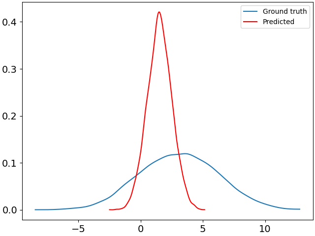
They don’t really match. Is there something I’m missing?

In addition, is there a way to sample a large amount of points at once from a function such as test_data? Of note is that calling methods on the generated distribution object wouldn’t really work, because the “center” parameter would be sampled only once.

Thanks

you’re missing the following (at least):

  • presumably you want center = npy.sample("center", c_dist) outside the plate not inside (you have one center for each datapoint, which is why your result is heavily regularized towards zero)
  • you didn’t include observation noise in your plot

there are various ways to sample distributions in batches, including plates.

Thank you for your response,

It seems to be that the sample being inside the plate is correct. I do want each sample to have a different center. The “test_data” distribution is regenerated for each point to achieve this.

I’ll note that if I don’t regenerate the distribution for each sample, (the center is picked once), and move the center sample out of the plate, it does fit pretty nicely. But that’s not the distributions I’m trying to fit.

I’m not sure what you mean by this, or how to achieve it. But I am interested in learning more.

I know how to sample a Distribution in a batch, by providing the sample_shape arg to sample. However, this doesn’t allow me to say, vary the center per-sample (as I’m doing here. I’m interested specifically about sampling a function that returns distributions.

Thanks

well in that case you presumably want something like

npy.param("a", jnp.zeros(len(data)))
npy.param("b",  jnp.ones(len(data)), ...)

Wouldn’t that make the a and b be separate for each sample? I want the param() to be a single value, but sample() to be unique to each sampled value. You did give me an idea though:

center = npy.sample(
  "center",
  c_dist,
  sample_shape=(len(data),),
)

This unfortunately did not work.

To clarify, the behavior I desire is:

  • All evaluations use the same param values “a” and “b”
  • However, every evaluation should use a different sample values “center”

i think you may have some misunderstanding about your model and the corresponding posterior.

if center is a local latent variable then in the posterior the posterior over the len(data)-many centers is a multivariate distribution in which each marginal is, in general, different. consequently if you’re doing variational inference and want to recover a reasonably accurate posterior you need to provide a variational family (a guide) that reflects that (and not one that is severely restricted by lots of parameter sharing)

The guide has the exact structure of the function that generated the observations (unless I’m mistaken). There are many "center"s in the generator function. I believe there are also many "center"s in guide (again, unless I’m mistaken). However, your suggestion above was regarding “a” and “b”, of which there should be only one, shared among all observations.

Is the guide more “restricted” than the generative function? If so, how so?

Thanks

i think it might be helpful if you write out an equation for the joint density of the model you want. then you can write down an equation for the joint density of the variational family you want. then we can talk about translating that into numpyro code

I’m not confident I can write that equation correctly (I tried googling about it but no luck. If you point me to a reference I can try). But I can write you some small generative functions, which I believe will get point across.

import random as r


def prior():
    center = r.gauss(0, 1)
    return r.gauss(center, 1)


def posterior(a, b):  # a and b are params, and the same for every sample
    center = r.gauss(a, b)  # however the center changes per-sample
    return r.gauss(center, 1)

Thanks

a generative story in words would be fine but could you please be more specific?

e.g.

  1. sample a single scalar center ~ normal(0, 1)
  2. for i=1,…,N sample x_i ~ normal(center, scale_obs)

versus

  1. for i=1,…,N sample center_i ~ normal(0, 1)
  2. for i=1,…,N sample x_i ~ normal(center_i, scale_obs)

I mean the second option, so, for the model:

  1. for i=1,…,N sample center_i ~ normal(0, 1)
  2. for i=1,…,N sample x_i ~ normal(center_i, 1)

For the posterior (where A and B are params):

  1. for i=1,…,N sample center_i ~ normal(A, B)
  2. for i=1,…,N sample x_i ~ normal(center_i, 1)

the thing is that if A and B are scalars, that family of distributions cannot recover the true posterior. at best it can recover an approximation. because like i said above:

if center is a local latent variable then in the posterior the posterior over the len(data) -many center s is a multivariate distribution in which each marginal is, in general, different. consequently if you’re doing variational inference and want to recover a reasonably accurate posterior you need to provide a variational family (a guide) that reflects that (and not one that is severely restricted by lots of parameter sharing)

so i’m not sure why you would want to do that. do you have a specific reason? note also that for simple models like that it’s generally a better idea to use HMC. is there a particular reason you want to use SVI?

I guess my question then becomes how would I, in general, write a posterior guide given that I know the exact structure of the distribution the data comes from.

Because I want to infer the true values of the variables a and b. I was under the impression that MCMC could not be used in this manner.

After reading a bit of the MCMC tutorial again and testing it out, by transforming my params a and b into samples of normal distributions, it seems to give me good results. With:

def model():
    a = npy.sample("a", Normal(0.0, 1.0))
    b = npy.sample("b", Normal(1.0, 1.0))
    c_dist = Normal(a, b)
    with npy.plate("observations", len(data)):
        center = npy.sample("center", c_dist)
        npy.sample(f"result", Normal(center, 1.0), obs=data)

I can then use jnp.average(mcmc.get_samples()['a']) and jnp.average(mcmc.get_samples()['b']) as estimates of the true values of a and b.

An important question: what is the MCMC equivalent of ELBO? In other words, how do I know if my model is good? Optimally, this would be a single number I can compare.

Thanks

there is no simple answer here. even in the context of SVI just because your ELBO trends towards a large value doesn’t mean your model is good (though it may mean that your optimization has converged).

in terms of whether MCMC samples are likely to be reasonably good approximations of samples from the true posterior, look at the r_hat metric provided by numpyro. ideally all your r_hats should be < 1.05ish