Hi
I would like to generate a simple “error in (feature) variable model”. This kind of models is required when the x and y values are subject to errors (not only the y values like in typical mean squared error minimization).
On the long run this model shall be non-linear, e.g. a Bayesian neural network.
However, I start out with a simple toy test-case where I use a simple linear Regression (which has a well known optimal solution).
In Maximum-Likelihood estimation the optimal linear model is described by an adapted loss function, see Deming Regression: Deming regression - Wikipedia

Key here is that the observed (x_i,y_i) training pairs are described as having errors themselves: (x_i,y_i)=(x_i^*+\eta_i,y_i^*+\epsilon_i)
So there is “error-free” (x_i^*, y_i^*=y_\theta(x_i^*)) associated with each training example. While the function y_\theta(x_i^*) is fitted by finding the most likely parameters \theta, finding all the optimal measurement x_i^* needs to be added to the optimization problem.
I want to create a Bayesian version of Deming regression which can then be easily generalized to nonlinear models later.
Here is what I have so far:
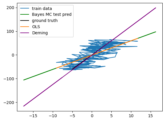
The problem is, that the x_i*=x_i-error\_bias_i - or equivalently the (for each sample constant but arbitrary) error_bias is not correctly fitted (it just stays at it’s initialization value) when I use the NUTs MCMC or the SVI approach with autoguide = pyro.infer.autoguide.AutoDelta(model)
Therefore, the model (as well as ordinary least squares) is not able to reproduce the optimal (Deming regression) solution, which coincides with the ground truth of the generating process):
Could you please help me to get this work with pyro? I would already be happy with solving the linear case correctly.
Later I would want to
- optimze a non-linear model like a neural network in a later stage
- assume that the errors in x and y may be depending on x and may be heteroscedastic (i.e. we might have varying distributions of errors in both x and y)
If you have any furhter hints for the generalization, I would also be very happy!
Below you find my code (unfortunately, I could not upload my jupyter notebook).
import matplotlib.pyplot as plt
import torch
import copy
x1 = torch.rand(50, 1) * 0.3 - 1
x2 = torch.rand(50, 1) * 0.5 + 0.5
x_no_error=torch.cat([x1,x2])
num=200
x_no_error = torch.linspace(-5,5, steps=num).unsqueeze(1)
gt_slope=12
gt_intercept=0
def f(x_no_error, noise=True):
y=torch.cos(x_no_error*4+0.8)
y=gt_slope*x_no_error+gt_intercept
x=copy.deepcopy(x_no_error)
if noise:
y+= 5* torch.randn_like(x_no_error)
x+=3 * torch.randn_like(x_no_error)
return x,y
x,y=f(x_no_error)
x_test_no_error = torch.linspace(-10, 10, 401).unsqueeze(-1)
x_test,y_test=f(x_test_no_error)
plt.plot(x,y)
import pyro
pyro.enable_validation(True)
import pyro.distributions as dist
def prediction(offset, slope, x_mu_obs):
y_pred = offset + slope * x_mu_obs
return y_pred
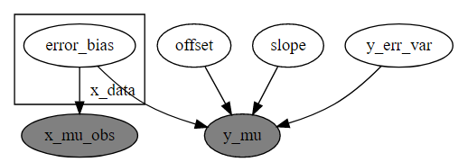
def model(x, y):
with pyro.plate("x_data", len(x)):
error_bias=pyro.sample("error_bias", dist.Normal(0, 2)) #only initial guess???
x_no_error_estimated=x-error_bias
x_mu_obs = pyro.sample('x_mu_obs', dist.Normal(x_no_error_estimated, 0.1), obs=x)
offset = pyro.sample('offset', dist.Normal(0, 10))
slope = pyro.sample('slope', dist.Normal(0, 10))
y_pred = prediction(offset, slope, x_no_error_estimated)
y_err_var = pyro.sample('y_err_var', dist.HalfNormal(5.))
y_obs = pyro.sample('y_mu', dist.Normal(y_pred, y_err_var), obs=y)
return x_mu_obs, y_obs
pyro.render_model(model, model_args=(x,y), render_params=True)
import torch
from pyro.infer import MCMC, NUTS
# Convert x and y to PyTorch tensors
x = torch.tensor(x)
y = torch.tensor(y)
# Run MCMC using NUTS
nuts_kernel = NUTS(model)
mcmc = MCMC(nuts_kernel, num_samples=201, warmup_steps=200, num_chains=1)
mcmc.run(x, y) #fits the model to the observations
# Get posterior samples
samples = mcmc.get_samples()
# Get posterior predictive samples
predictive = pyro.infer.Predictive(model, posterior_samples=samples)
result = predictive(torch.squeeze(x),torch.squeeze(y))
y_test_pred=prediction(samples["offset"].mean(), samples["slope"].mean(), x_test)
# Plot for control
import numpy as np
from scipy.odr import ODR, Model, Data
# Define the model
def line_model(p, x):
a, b = p
return a*x + b
# Create the ODR object
model_deming = Model(line_model)
data = Data(x[:,0], y[:,0])
odr = ODR(data, model_deming, beta0=[1, 1])
# Perform the orthogonal regression
result = odr.run()
# Print the result
print("Deming Intercept: ", result.beta[1])
print("Deming Slope: ", result.beta[0])
print("Standard deviation of the estimates: ", result.sd_beta)
from sklearn.linear_model import LinearRegression
ols_linreg_model = LinearRegression()
ols_linreg_model.fit(x, y[:,0]);
plt.plot(x,y, label="train data")
plt.plot(x_test,y_test_pred, label="Bayes MC test pred", color = "green") #XXX not learning deming
plt.plot(*f(x_no_error, noise=False), label="ground truth", color = "black")
plt.plot(x, ols_linreg_model.predict(x), label="OLS")
plt.plot(x_test,result.beta[1]+result.beta[0]*x_test, label="Deming", color="purple")
plt.legend()
PS: I also had a look at what others did e.g. in pymc: Errors-in-variables model in PyMC3 - Questions - PyMC Discourse However, I need to note that their model fails to reproduce the Deming regression solution as well!