Does SVI converges towards the right solution? (4-parameters MVN)

campagne · December 12, 2021, 1:21pm

Hello,
The question of the good convergence of the SVI arises looking at a simple exercice. Here is the complete snippet:

import jax
import jax.numpy as jnp
from jax.config import config
config.update("jax_enable_x64", True)

import numpy as np
import matplotlib as mpl
import matplotlib.pyplot as plt
mpl.rc('image', cmap='jet')
mpl.rcParams['font.size'] = 18
mpl.rcParams["font.family"] = "Times New Roman"

import corner
import arviz as az

import numpyro
from numpyro.diagnostics import hpdi
import numpyro.distributions as dist
from numpyro import handlers
from numpyro.infer import MCMC, NUTS, init_to_sample

numpyro.util.enable_x64()

# Get mock data
param_true = np.array([1.0, 0.0, 0.2, 0.5, 1.5])
sample_size = 5_000
sigma_e = param_true[4]          # true value of parameter error sigma
random_num_generator = np.random.RandomState(0)
xi = 5*random_num_generator.rand(sample_size)-2.5
# do not produce noisy data to get theoretical contours
yi = param_true[0] + param_true[1] * xi + param_true[2] * xi**2 + param_true[3] *xi**3
plt.hist2d(xi, yi, bins=50);

####
# Build Numpyro model
####
def my_model(Xspls,Yspls=None):
    a0 = numpyro.sample('a0', dist.Normal(0.,10.))
    a1 = numpyro.sample('a1', dist.Normal(0.,10.))
    a2 = numpyro.sample('a2', dist.Normal(0.,10.))
    a3 = numpyro.sample('a3', dist.Normal(0.,10.))

    mu = a0 + a1*Xspls + a2*Xspls**2 + a3*Xspls**3

    return numpyro.sample('obs', dist.Normal(mu, sigma_e), obs=Yspls)

###
# NUTS sampling to compare with the Truth and the SVI sampling
###
# Start from this source of randomness. We will split keys for subsequent operations.
rng_key = jax.random.PRNGKey(0)
_, rng_key, rng_key1, rng_key2 = jax.random.split(rng_key, 4)


# Run NUTS.
kernel = NUTS(my_model, init_strategy=numpyro.infer.init_to_median())
num_samples = 10_000
n_chains = 1
mcmc = MCMC(kernel, num_warmup=1_000, num_samples=num_samples,  
            num_chains=n_chains,progress_bar=True)
mcmc.run(rng_key, Xspls=xi, Yspls=yi)
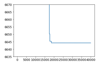
mcmc.print_summary()
samples_nuts = mcmc.get_samples()

#####
# SVI 
#####
import numpyro.infer.autoguide as autoguide
from numpyro.infer import Predictive, SVI, Trace_ELBO, TraceMeanField_ELBO
from numpyro.optim import Adam

guide = autoguide.AutoMultivariateNormal(my_model, init_loc_fn=numpyro.infer.init_to_sample())
optimizer = numpyro.optim.Adam(step_size=5e-3)
svi = SVI(my_model, guide,optimizer,loss=Trace_ELBO())
svi_result = svi.run(jax.random.PRNGKey(0), 10000, Xspls=xi, Yspls=yi)

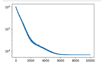
Now, ploting the loss

plt.plot(svi_result.losses)
plt.yscale('log')

gets a reasonable behaviour

So one gets samples from SVI optimized guide

samples_svi = guide.sample_posterior(jax.random.PRNGKey(1), svi_result.params, sample_shape=(5000,))

What about the result of the linear least square fit

Y = yi[:,np.newaxis]   # output (N,1)
X = np.vstack((np.ones(sample_size),xi,xi**2,xi**3)).T   # input features (N,4)
K = X.T @ X
Theta_hat= (np.linalg.inv(K) @ X.T @ Y).squeeze()  # fitted theta vector Y=X @ Theta 
Sigma_theta = sigma_e**2 * np.linalg.inv(K)   # Covariance of Theta

One gets Theta_hat = true vector

array([1.00000000e+00, 2.52575738e-15, 2.00000000e-01, 5.00000000e-01])

Get samples from MVN with loc=Theta_hat and cov mtx = Sigma_theta

dist_theta = dist.MultivariateNormal(loc=Theta_hat, covariance_matrix=Sigma_theta)
samples_true = dist_theta.sample(jax.random.PRNGKey(42), (100_000,))
spl_true = {labels[i]:samples_true[:,i] for i in range(len(labels))}

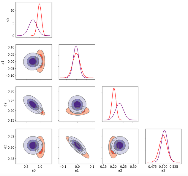
Now plot 1D and 2D Kde plots of

spl_true: a sampling from the LSQ fit  in red which leads to MVN distrib
samples_nuts: the NUTS sampling of the model  in blue
samples_svi:  The SVI sampling from a MVN guide optimized on model in green

labels = [*samples_nuts]
ax = az.plot_pair(
    spl_true,
    kind="kde",
    var_names=labels,
    kde_kwargs={
        "hdi_probs": [0.3, 0.6, 0.9],  # Plot 30%, 60% and 90% HDI contours
        "contourf_kwargs": {"cmap": "Reds"},
    },
    marginals=True, textsize=20,
);
az.plot_pair(
    samples_nuts,
    kind="kde",
    var_names=labels,
    kde_kwargs={
        "hdi_probs": [0.3, 0.6, 0.9],  # Plot 30%, 60% and 90% HDI contours
        "contourf_kwargs": {"cmap": "Blues", "alpha": 0.2}, 
        "plot_kwargs":{"color":"blue"}
    },
    marginals=True, textsize=20,ax=ax
);
az.plot_pair(
    samples_svi,
    kind="kde",
    var_names=labels,
    kde_kwargs={
        "hdi_probs": [0.3, 0.6, 0.9],  # Plot 30%, 60% and 90% HDI contours
        "contourf_kwargs": {"cmap": "Greens", "alpha": 1.0}, 
        "plot_kwargs":{"color":"green"}
    },
    marginals=True, textsize=20,ax=ax
);

Here is the result

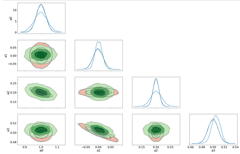
The NUTS sampling agrees very well with the Lsq Fit ones (the two sets of contours 1D/2D are barely distinguishable)

But the SVI (green) contours (and 1D pdf too) are quite different and I do not understand why there are such as the true posterior pdf is a MVN so it is the same distribution family as the guide distrib. So, is there a problem of convergence even in this 4-parameters very simple exercice?

fehiepsi · December 12, 2021, 4:13pm

Did you try a smaller learning rate and a larger svi step, says (1e-3 and 100000)?

campagne · December 12, 2021, 4:50pm

Ho! Got it

The new loss is 6648.6333 compared to 6652.8623 !!! so the difference is very small compared to inity loss about 1017751.20 But the Kde plots are now matching the truth !!! Unbelievable !

martinjankowiak · December 12, 2021, 6:21pm

generally speaking the only way to achieve approximate convergence with these kinds of algorithms is to decrease the learning rate towards zero. e.g. start at 0.01, then lower to 0.001, and keep lowering until 0.0001 or 0.00001—all depending on details, how much compute you want to spend, etc. in other words a large number of iterations at a largeish learning rate generally does not suffice

campagne · December 12, 2021, 6:30pm

Yes for sure @martinjankowiak, I daily use Pytorch for CNN. But here the SVI loss difference between the two optimized SVI is so small that I cannot see a way (of a more complex example) to decide that the optimal loss is reached, as usually there are fluctuations arround the global minimum. But this simple exo is rich of outcomes to practice SVI correctly. Thanks

campagne · December 13, 2021, 9:18am

Hi @fehiepsi and @martinjankowiak

I have a addendum which also answers a question I had sometimes ago: does the SVI guide optimized leading to the lowest loss, is really the best guide? So lets us takes my favourite exercise described above, and use this snippet:

First use a code to keep the history of the loss, and the guide with the lowest loss. This is very similar to Neural Network optimisation where we keep track of the validation test loss and keep the model that leads to the minimum loss during the optimisation.

from functools import partial

def body_fn(i,carry):
    svi_state, svi_state_best, losses = carry
    svi_state, loss =svi.update(svi_state,Xspls=xi, Yspls=yi)

    def update_fn(x):
        return losses.at[i].set(loss), svi_state
    def keep_fn(x):
        return losses.at[i].set(losses[i-1]), svi_state_best
    losses, svi_state_best = jax.lax.cond(loss<losses[i-1],update_fn,keep_fn,None)
    return (svi_state, svi_state_best, losses)

Proceed to the SVI optimisation

svi_state = svi.init(jax.random.PRNGKey(42),Xspls=xi, Yspls=yi)
num_steps=40_000
losses = jnp.zeros(num_steps)
losses = losses.at[0].set(1e10)
svi_state_best = svi_state
carry = (svi_state,svi_state_best,losses)
carry = jax.lax.fori_loop(1,num_steps,body_fn,carry)

Plot the loss steping

plt.plot(carry[2])
plt.ylim([6635,6670])

You will get this plot and see that the minimum loss is 6644 so below the 6648 mentioned above for the SVI guide which agrees with the theretical contours:

Now get the samples of this guide (lowest loss)

samples_lowest_loss = guide.sample_posterior(jax.random.PRNGKey(1),svi.get_params(carry[1]), 
                                      sample_shape=(100_000,))

and now compare the Theoretical contours in Reds with the contours from this guide (lowest loss) in Purples

ax = az.plot_pair(
    spl_true,
    kind="kde",
    var_names=labels,
    kde_kwargs={
        "hdi_probs": [0.3, 0.6, 0.9],  # Plot 30%, 60% and 90% HDI contours
        "contourf_kwargs": {"cmap": "Reds"},
    },
    marginals=True, textsize=15,
    figsize=(15, 15),
    marginal_kwargs={"color": "red"}
);
az.plot_pair(
    samples_lowest_loss,
    kind="kde",
    var_names=labels,
    kde_kwargs={
        "hdi_probs": [0.3, 0.6, 0.9],  # Plot 30%, 60% and 90% HDI contours
        "contourf_kwargs": {"cmap": "Purples", "alpha": 1.0}, 
    },
    marginals=True, textsize=15,
    marginal_kwargs={"color": "purple"},
    ax=ax
);

The result is clear: the SVI guide with the lowest loss (at least in early phase of Adam optimisation) is not guaranteed to give the true contours !

I think this exercise is very enlightening.

fehiepsi · December 13, 2021, 12:56pm

Typically you will want to set num_particles in the constructor of TraceElbo to a large value if you want to get robust result. Otherwise, the loss is stochastic so the smallest one might not be the best.

campagne · December 16, 2021, 10:10am

Ok Thanks @fehiepsi. In present case increasing the number of steps and decreasing the step_size of Adam minimizer gives perfect posteriors.

Now, is is possible to get an AutoGuide similar to AutoMVN but with a specification of covariance per blocks ? For instance if in my original model I have {“a0”, “a1”,“a2”,“a3”,“a4”,“a5”,“a6”} I would for instance makes a block 3x3 for {a0, a1, a2} an other one 2x2 for {a4,a5} and diagonal for {a3} and {a6} and the other elements of the 7x7 Cov Mtx to be 0 ?
In a sense this is similar to NUTS dense_mass specification.

fehiepsi · December 16, 2021, 1:04pm

Currently, we don’t have AutoStructured in numpyro but should be possible (this is in our plan but does not have timeline for it yet) after ProvenanceArray is available. For now, you might want to use the Pyro version to explore the ideas. I think the settings that you need for

a block 3x3 for {a0, a1, a2} an other one 2x2 for {a4,a5} and diagonal for {a3} and {a6} and the other elements of the 7x7 Cov Mtx to be 0

is

guide = AutoStructured(
    model=model,
    conditionals={"a0": "normal", ..., "a6": "normal", remaining: "delta"},
    dependencies={
        "a1": {"a0": "linear"},
        "a2": {"a0": "linear", "a1": "linear"},
        "a5": {"a4": "linear"},
)

campagne · December 16, 2021, 1:29pm

Hum, so I should change the code from Numpyro to Pyro…
Anyway I am looking for more AutoGuideMVN with Covariance matrix shape tunable Thanks