Difference between the methods to compute potential energy

I computed the potential energy corresponding to a model. I have used two methods to do so:

  1. Using extra_fields=('potential_energy',) in mcmc.run
  2. Using potential_energy under numpyro.infer.util

But, in both cases, I am getting different values. Can you please elaborate more about both method and their specific use?

Further, I also used log_density under numpyro.infer.util which gave me results same as that obtained using (1.) with a negative sign but with different digits post decimal. Isn’t log_density = -potential_energy or am I missing out on something?

Almost! Log density is the “real” measure that we care about, i.e. the log of the probability function, while potential energy is that same value after a co-ordinate transformation to the “unconstrained domain”. If your parameters have discontinuous or constrained priors, like Uniform or HalfNormal, they need to be re parameterized internally to something that’s smooth and differentiable for some algorithms, e.g. MCMC, to work properly. To transform between the two, all you have to do is multiply by the Jacobian of the transformation between constrained and unconstrained.

Regarding the differences in potential energy between utils and the MCMC chain, the problem is that potential_energy expects inputs in unconstrained form. When getting potential_energy as an extra_field in an MCMC run, this is automatically being done under the hood.

You can perform the transformation using something like:

transforms = {"x": numpyro.distributions.biject_to(x_prior.support)}  
  
x_con = np.linspace(0, 2, 1024)  
x_uncon = transform_fn(transforms, {'x': x_con}, invert=True)['x']  

Where x_prior is whatever prior distribution you used to define ‘x’ in your model, e.g. numpyro.distributions.Uniform(-1,1).

1 Like

Here’s a little diagram of how you can switch between the different functions and what inputs they need.

The example graphs are for a simple model:

\pi(x) = Uniform(-1,1), \;\;\; \mathcal{L}(x) = (1+x)(1-x)

I don’t know the exact reparameterization NumPyro uses, but in this mock-up I’ve used:

z = \text{atanh}(x)

image

You can see how this goes from a constrained domain, x \in [-1,1], to an unconstrained domain, z \in (-\infty, \infty), which means any MCMC sampler navigating in z-space wouldn’t need to worry about sharp cliffs at the domain boundaries.

2 Likes

Thank you for the fantastic explanation. Based on your writeup, won’t the potential_energy in the unconstrained space be equivalent to the log_density in the constrained space? If so, then why have you added an extra adjustment term in the form of log jacobian while comparing potential_energy and log_density in the diagram?

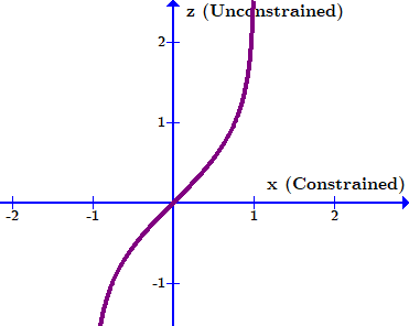
Note quite, because the probability density changes as you shift between coordinates. The core idea here is they are densities, and so equivalent differential elements need to have the same total power contained within them. E.g., if I have some constrained parameter x that converts to unconstrained parameter z, I need:

P_x(x) dx = P_z(z) dz

Which of course rearranges to:

P_x(x) \cdot\frac{dx}{dz} = P_z(z) \\ \ln \vert P_x(x) \vert + \ln \vert \frac{dx}{dz}\vert = \ln \vert P_z(z)\vert

I.e. to go between the two log-densities I need to add a log of the derivative.

If I have many parameters being transformed, like:

x_1 \rightarrow z_1(x_1) \\ x_2 \rightarrow z_2(x_2) \\ \vdots \\

I need to correct by the product of all of these:

\ln \vert P_z(z)\vert = \ln \vert P_x(x) \vert + \ln \vert \frac{dx_1}{dz_1} \frac{dx_2}{dz_2} \dots \vert

And in the more general case where the transformed parameters “mix”, i.e.:

x_1 \rightarrow z_1(x_1, x_2 \dots) \\ x_2 \rightarrow z_2(x_1, x_2 \dots) \\ \vdots \\

The correction factor is the determinant of the Jacobian of all of these transformations:

J = \left[ \matrix{{\frac{\partial z_1}{\partial x_1},\frac{\partial z_1}{\partial x_2}}\\{\frac{\partial z_2}{\partial x_1},\frac{\partial z_2}{\partial x_2}}} \right]
\ln \vert P_z(z)\vert = \ln \vert P_x(x) \vert + \ln \vert det(J) \vert

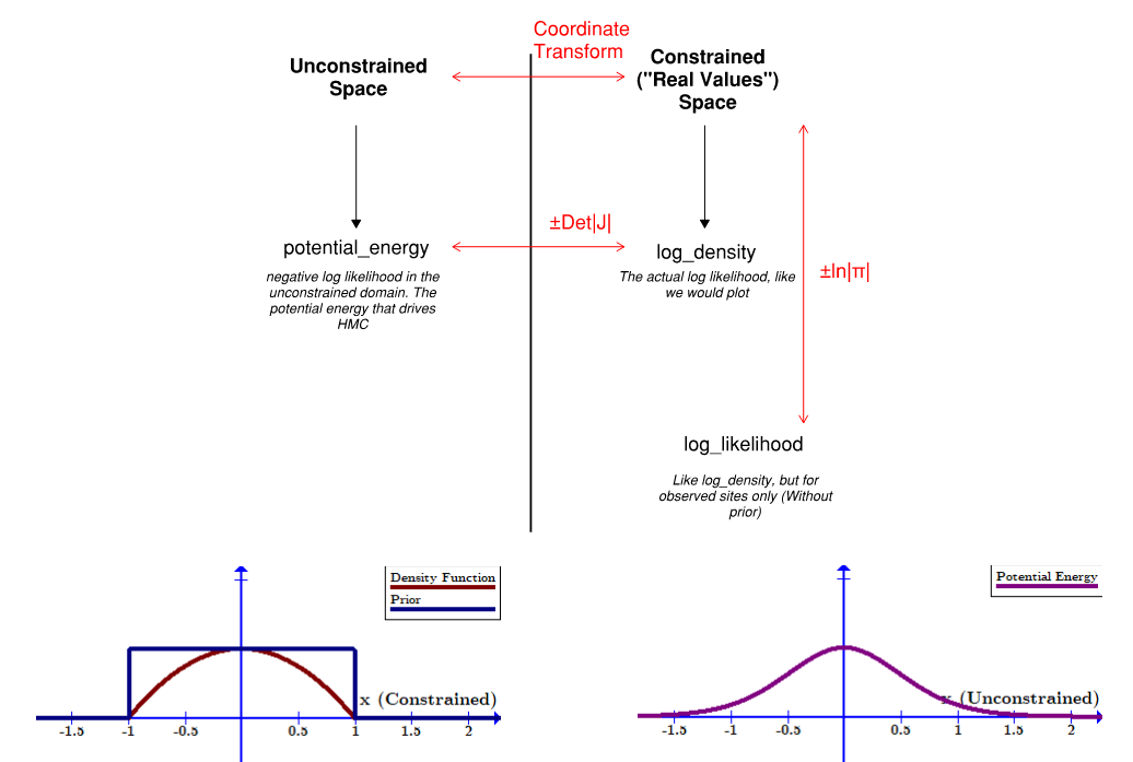
Throw in a negative or two to account for inverses and the difference between density and potential energy, and you have a clearer picture

1 Like

Thanks for such a comprehensive explanation :grinning: